1 Correlation

1.1 Correlation and Causation

1.2 Pearson correlation coefficient

Pearson correlation coefficient ($r$) is a measure of the strength and the direction of a linear relationship between two variables in the sample,

\[r=\frac{\sum(x_{i} -\bar{x})(y_{i} -\bar{y}) }{\sqrt{\sum (x_{i} -\bar{x})^{2} \sum (y_{i} -\bar{y})^{2} } } \]

where $r$ always lies between -1 and 1. Values of $r$ near -1 or 1 indicate a strong linear relationship between the variables whereas values of $r$ near 0 indicate a weak linear relationship between variables. If $r$ is zero the variables are linearly uncorrelated, that is there is no linear relationship between the two variables.

1.3 Hypothesis testing for the population correlation coefficient $\rho$

Hypothesis testing for the population correlation coefficient $\rho$.

Assumptions:

The sample of paired $(x, y)$ data is a random sample.
The pairs of $(x, y)$ data have a bivariate normal distribution.

The null hypothesis

$H_0: \rho = 0$ (no significant correlation)

against one of the alternative hypotheses:

$H_1: \rho \neq 0$ (significant correlation) ``Two-tailed test’’
$H_1: \rho < 0$ (significant negative correlation) ``Left-tailed test’’
$H_1: \rho > 0$ (significant positive correlation) ``Right-tailed test’’

Compute the value of the test statistic: \[t=\frac{r\; \sqrt{n-2} }{\sqrt{1-r^{2} } }\sim T_{(n-2)} \;\; \text{with}\;\; df = n-2. \]

where $n$ is the sample size.

The critical value(s) for this test can be found from T distribution table ( $\pm t_{\alpha/2}$ for a two-tailed test, $- t_{\alpha}$ for a left-tailed test and $t_{\alpha}$ for a right-tailed test).

If the value of the test statistic falls in the rejection region, then reject $H_0$; otherwise, do not reject $H_0$.
Statistical packages report p-values rather than critical values which can be used in testing the null hypothesis $H_0$.

1.4 Correlation and linear transformation

Suppose we have a linear transformation of the two variables $x$ and $y$, say $x_1=a x+b$ and $y_1=cy+d$ where $a>0$ and $c>0$. Then the Pearson correlation coefficient between $x_1$ and $y_1$ is equal to Pearson correlation coefficient between $x$ and $y$.
For our example, suppose we convert cars’ prices from dollars to pounds (say $\$1=$ , so $y_1=0.75 y$), and we left the age of the cars unchanged. Then we will find that the correlation between the age of the car and its price in pounds is equal to the one we obtained before (i.e. the correlation between the age and the price in dollars).
A special linear transformation is to standardize one or both variables. That is obtaining the values $z_x=(x-\bar{x})/s_x$ and $z_y=(y-\bar{y})/s_y$. Then the correlation between $z_x$ and $z_y$ is equal to the correlation between $x$ and $y$.

1.5 Spearman’s rho correlation coefficient ($r_s$)

When the normality assumption for the Pearson correlation coefficient $r$ cannot be met, or when one or both variables may be ordinal, then we should consider nonparametric methods such as Spearman’s rho and Kendall’s tau correlation coefficients.
Spearman’s rho correlation coefficient, $r_s$,can be obtained by first rank the $x$ values (and $y$ values) among themselves, and then we compute the Pearson correlation coefficient of the rank pairs. Similarly $-1\leq r_s \leq 1$, the values of $r_s$ range from -1 to +1 inclusive.
Spearman’s rho correlation coefficient can be used to describe the strength of the linear relationship as well as the nonlinear relationship.

1.6 Kendall’s tau ($\tau$) correlation coefficient

Kendall’s tau, $\tau$, measures the concordance of the relationship between two variables, and $-1\leq \tau \leq 1$.
Any pair of observations $(x_i, y_i)$ and $(x_j, y_j)$ are said to be concordant if both $x_i > x_j$ and $y_i > y_j$ or if both $x_i < x_j$ and $y_i < y_j$. And they are said to be discordant, if $x_i > x_j$ and $y_i < y_j$ or if $x_i < x_j$ and $y_i > y_j$. We will have $n(n-1)/2$ of pairs to compare.
The Kendall’s tau ($\tau$) correlation coefficient is defined as: \[\tau=\frac{\text{number of concordant pairs} - \text{number of discordant pairs}}{n(n-1)/2}\]

1.7 Used cars example

The table below displays data on Age (in years) and Price (in hundreds of dollars) for a sample of cars of a particular make and model.(Weiss,2012)

Price ($y$)	Age ($x$)
85	5
103	4
70	6
82	5
89	5
98	5
66	6
95	6
169	2
70	7
48	7

The Pearson correlation coefficient, \[r=\frac{\sum x_i y_i - (\sum x_i) (\sum y_i)/n }{\sqrt{ [\sum x^2_{i} -(\sum x_i)^2/n] [\sum y^2_{i} -(\sum y_i)^2/n] } } \] \[r=\frac{4732-(58)(975)/11}{\sqrt{(326-58^2/11)( 96129-975^2/11)}}=-0.924\] the value of $r=-0.924$ suggests a strong negative linear correlation between age and price.
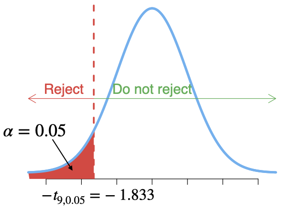
Test the hypothesis $H_0: \rho = 0$ (no linear correlation) against $H_1: \rho < 0$ (negative correlation) at significant level $\alpha=0.05$.

Compute the value of the test statistic: \[t=\frac{r\; \sqrt{n-2} }{\sqrt{1-r^{2} } }=\frac{-0.924\sqrt{11-2}}{\sqrt{1-(-0.924)^2}}=-7.249 \]

Since $t=-7.249<-1.833$, reject $H_0$.

1.8 Correlation in R

First we need to enter the data in R.

Price<-c(85, 103,  70,  82,  89,  98,  66,  95, 169,  70,  48)
Age<- c(5, 4, 6, 5, 5, 5, 6, 6, 2, 7, 7)
carSales<-data.frame(Price,Age)
str(carSales)

## 'data.frame':    11 obs. of  2 variables:
##  $ Price: num  85 103 70 82 89 98 66 95 169 70 ...
##  $ Age  : num  5 4 6 5 5 5 6 6 2 7 ...

Now let us plot age against price, i.e. a scatterplot.

plot(Price ~ Age, pch=16, col=2)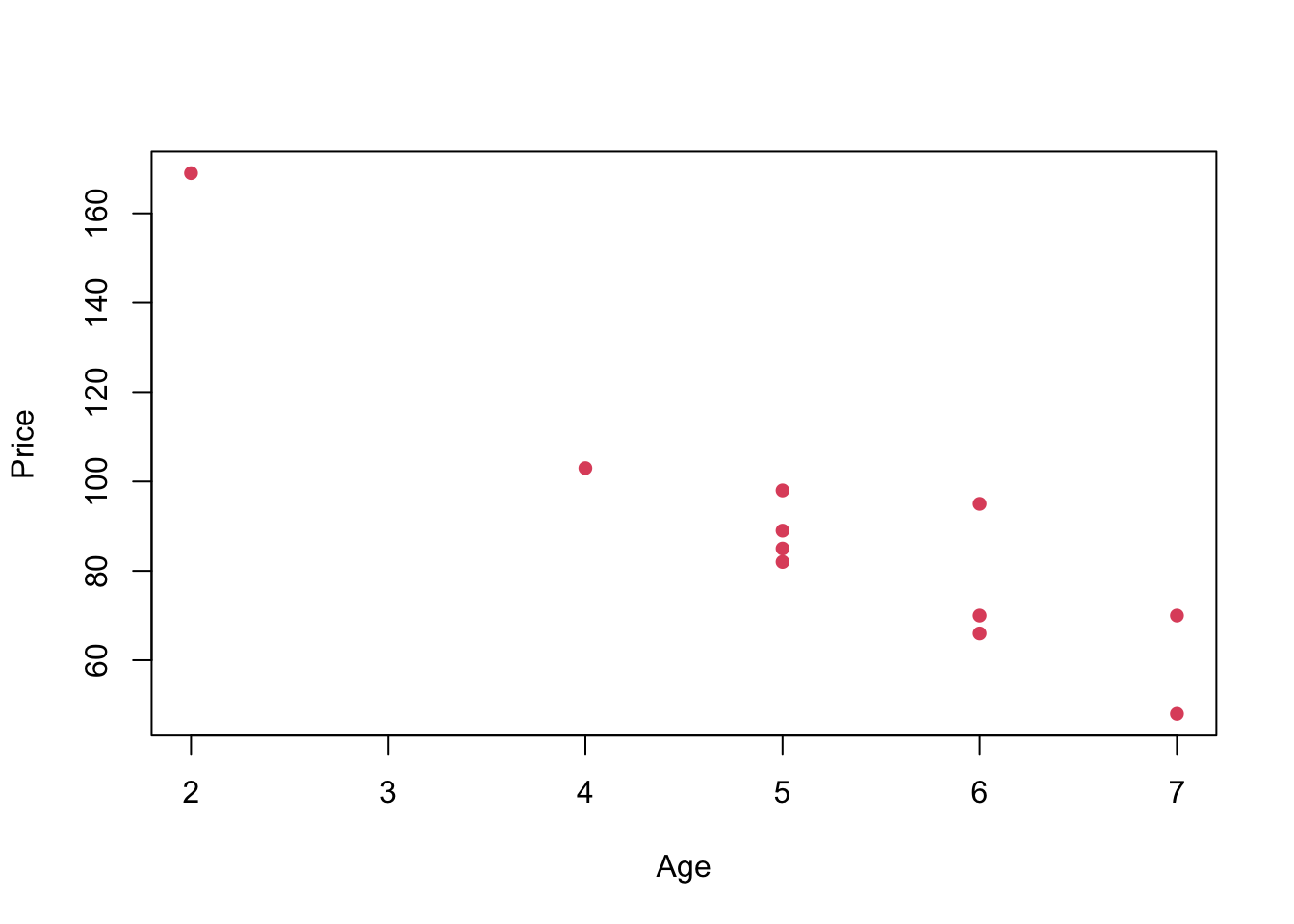

or we can use ggplot2 for a much nicer plot.

library(ggplot2)
# Basic scatter plot
ggplot(carSales, aes(x=Age, y=Price)) + geom_point()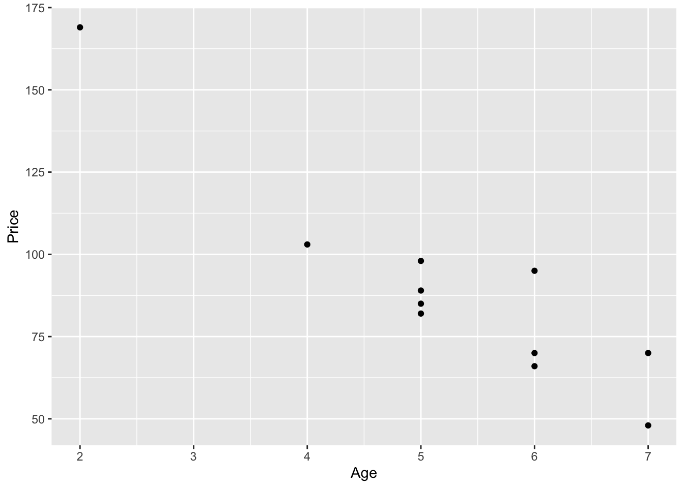

From this plot it seems that there is a negative linear relationship between age and price. There are several tools that can help us to measure this relationship more precisely.

cor.test(Age, Price,
         alternative = "less",
         method = "pearson", conf.level = 0.95)

## 
##  Pearson's product-moment correlation
## 
## data:  Age and Price
## t = -7.2374, df = 9, p-value = 2.441e-05
## alternative hypothesis: true correlation is less than 0
## 95 percent confidence interval:
##  -1.0000000 -0.7749819
## sample estimates:
##        cor 
## -0.9237821

Suppose now we scale both variables (standardized)

cor.test(scale(Age), scale(Price),
         alternative = "less",
         method = "pearson", conf.level = 0.95)

## 
##  Pearson's product-moment correlation
## 
## data:  scale(Age) and scale(Price)
## t = -7.2374, df = 9, p-value = 2.441e-05
## alternative hypothesis: true correlation is less than 0
## 95 percent confidence interval:
##  -1.0000000 -0.7749819
## sample estimates:
##        cor 
## -0.9237821

We notice that corr(age, price in pounds) $=$ corr(age, price in dollars).

We can also obtain Spearman’s rho and Kendall’s tau as follows.

cor.test(Age, Price,
         alternative = "less",
         method = "spearman", conf.level = 0.95)

## 
##  Spearman's rank correlation rho
## 
## data:  Age and Price
## S = 403.26, p-value = 0.0007267
## alternative hypothesis: true rho is less than 0
## sample estimates:
##        rho 
## -0.8330014

cor.test(Age, Price,
         alternative = "less",
         method = "kendall", conf.level = 0.95)

## 
##  Kendall's rank correlation tau
## 
## data:  Age and Price
## z = -2.9311, p-value = 0.001689
## alternative hypothesis: true tau is less than 0
## sample estimates:
##        tau 
## -0.7302967

As the p-values for all three tests (Pearson, Spearman, Kendall) less than $\alpha=0.05$, we reject the null hypothesis of no correlation between the age and the price, at the 5% significance level.

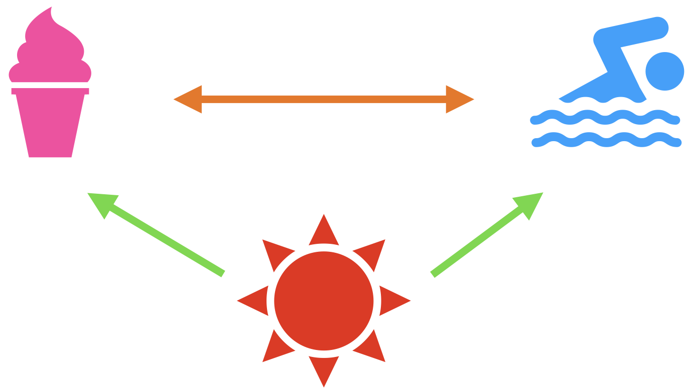
Now what do you think about correlation and causation?

https://xkcd.com/552/

2 Simple regression: Introduction

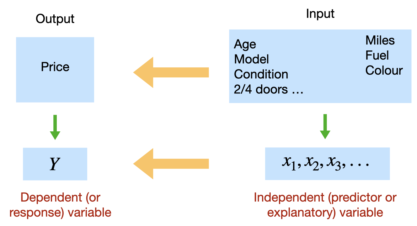
2.1 Motivation: Predicting the Price of a Used Car

2.2 Used cars example

The table below displays data on Age (in years) and Price (in hundreds of dollars) for a sample of cars of a particular make and model.(Weiss,2012)

Price ($y$)	Age ($x$)
85	5
103	4
70	6
82	5
89	5
98	5
66	6
95	6
169	2
70	7
48	7

2.3 Regression in R

First we need to enter the data in R.

Price<-c(85, 103,  70,  82,  89,  98,  66,  95, 169,  70,  48)
Age<- c(5, 4, 6, 5, 5, 5, 6, 6, 2, 7, 7)
carSales<-data.frame(Price,Age)
str(carSales)

## 'data.frame':    11 obs. of  2 variables:
##  $ Price: num  85 103 70 82 89 98 66 95 169 70 ...
##  $ Age  : num  5 4 6 5 5 5 6 6 2 7 ...

cor(Age, Price, method = "pearson")

## [1] -0.9237821

Scatterplot: Age vs. Price

library(ggplot2)
ggplot(carSales, aes(x=Age, y=Price)) + geom_point()

# Remove the confidence interval
ggplot(carSales, aes(x=Age, y=Price)) + 
  geom_point()+
  geom_smooth(method=lm, formula= y~x, se=FALSE)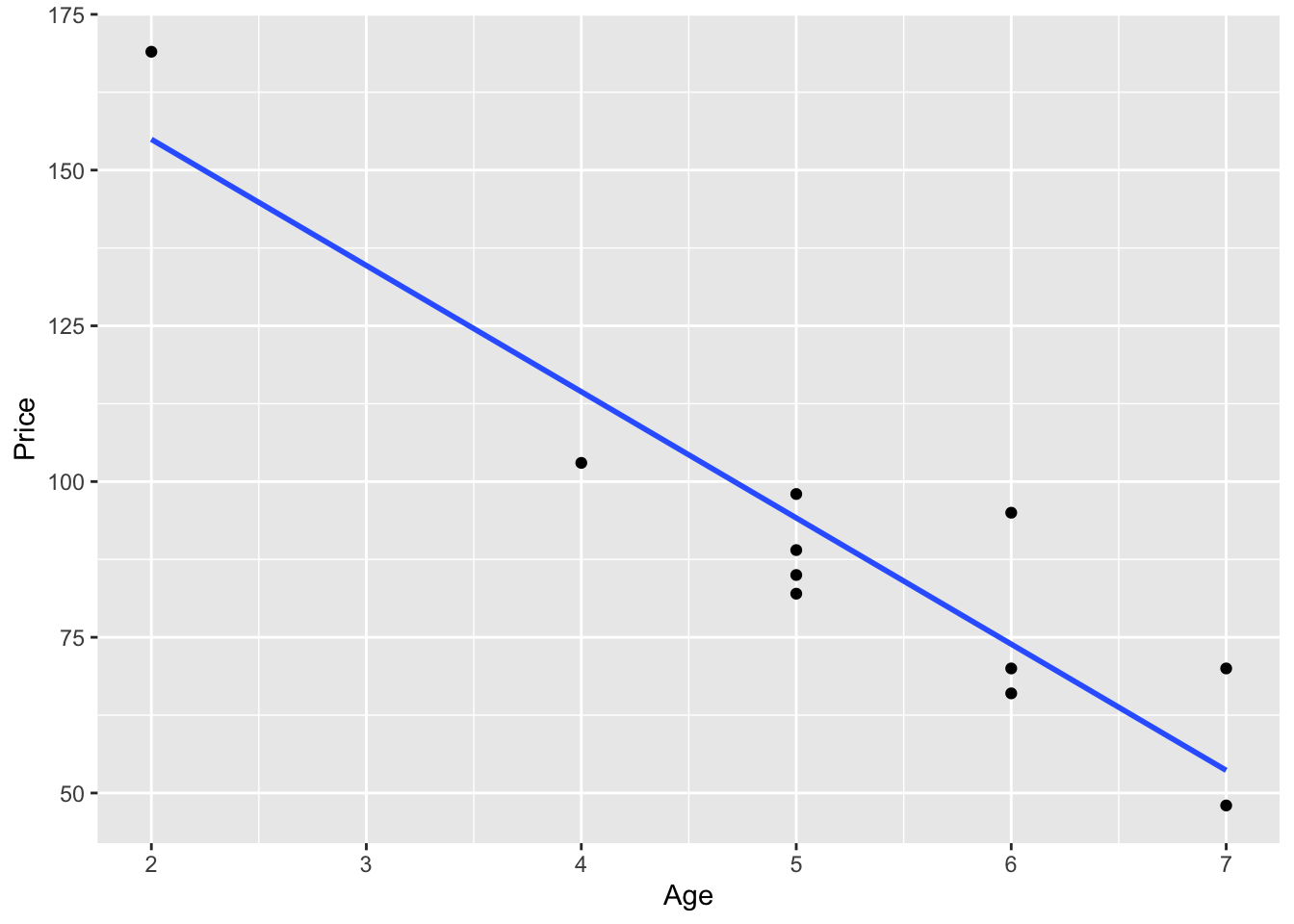

2.4 Simple linear regression

Simple linear regression (population) \[Y=\beta_0+\beta_1 x+\epsilon\] In our example: \[Price=\beta_0+\beta_1 Age+\epsilon\]

Simple linear regression (sample) \[\hat{y}=b_0+b_1 x\] where the coefficient $\beta_0$ (and its estimate $b_0$ or $\hat{\beta}_0$ ) refers to the $y$-intercept or simply the intercept or the constant of the regression line, and the coefficient $\beta_1$ (and its estimate (and its estimate $b_1$ or $\hat{\beta}_1$ ) refers to the slope of the regression line.

2.5 The Least-Squares criterion

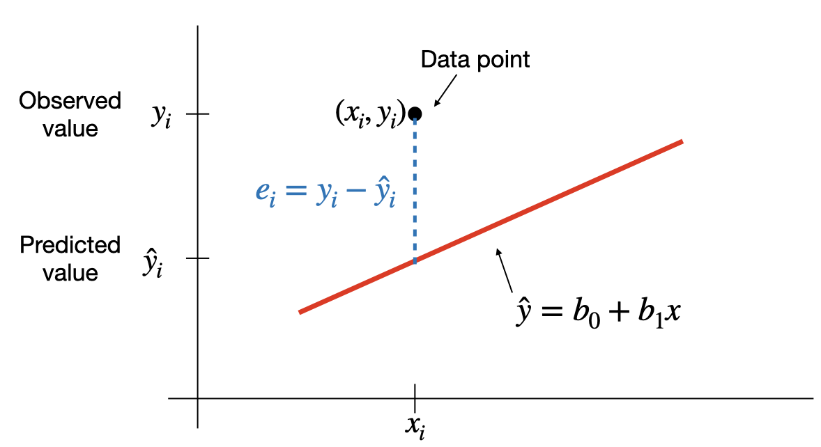
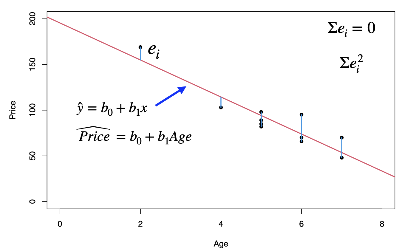
The least-squares criterion is that the line that best fits a set of data points is the one having the smallest possible sum of squared errors. The `errors’ are the vertical distances of the data points to the line.
The regression line is the line that fits a set of data points according to the least squares criterion.
The regression equation is the equation of the regression line.
The regression equation for a set of $n$ data points is $\hat{y}=b_0+b_1\;x$, where \[b_1=\frac{S_{xy}}{S_{xx}}=\frac{\sum (x_i-\bar{x})(y_i-\bar{y})}{\sum (x_i-\bar{x})^2} \;\;\text{and}\;\; b_0=\bar{y}-b_1\; \bar{x}\]
$y$ is the dependent variable (or response variable) and $x$ is the independent variable (predictor variable or explanatory variable).
$b_0$ is called the y-intercept and $b_1$ is called the slope.

2.6 SSE and the standard error

This least square regression line minimizes the error sum of squares \[SSE=\sum e^2_i =\sum (y_i-\hat{y}_i)^2\] The standard error of the estimate, $s_e=\sqrt{SSE/(n-2)}$, indicates how much, on average, the observed values of the response variable differ from the predicated values of the response variable.

2.7 Prediction

# simple linear regression
reg<-lm(Price~Age)
print(reg)

## 
## Call:
## lm(formula = Price ~ Age)
## 
## Coefficients:
## (Intercept)          Age  
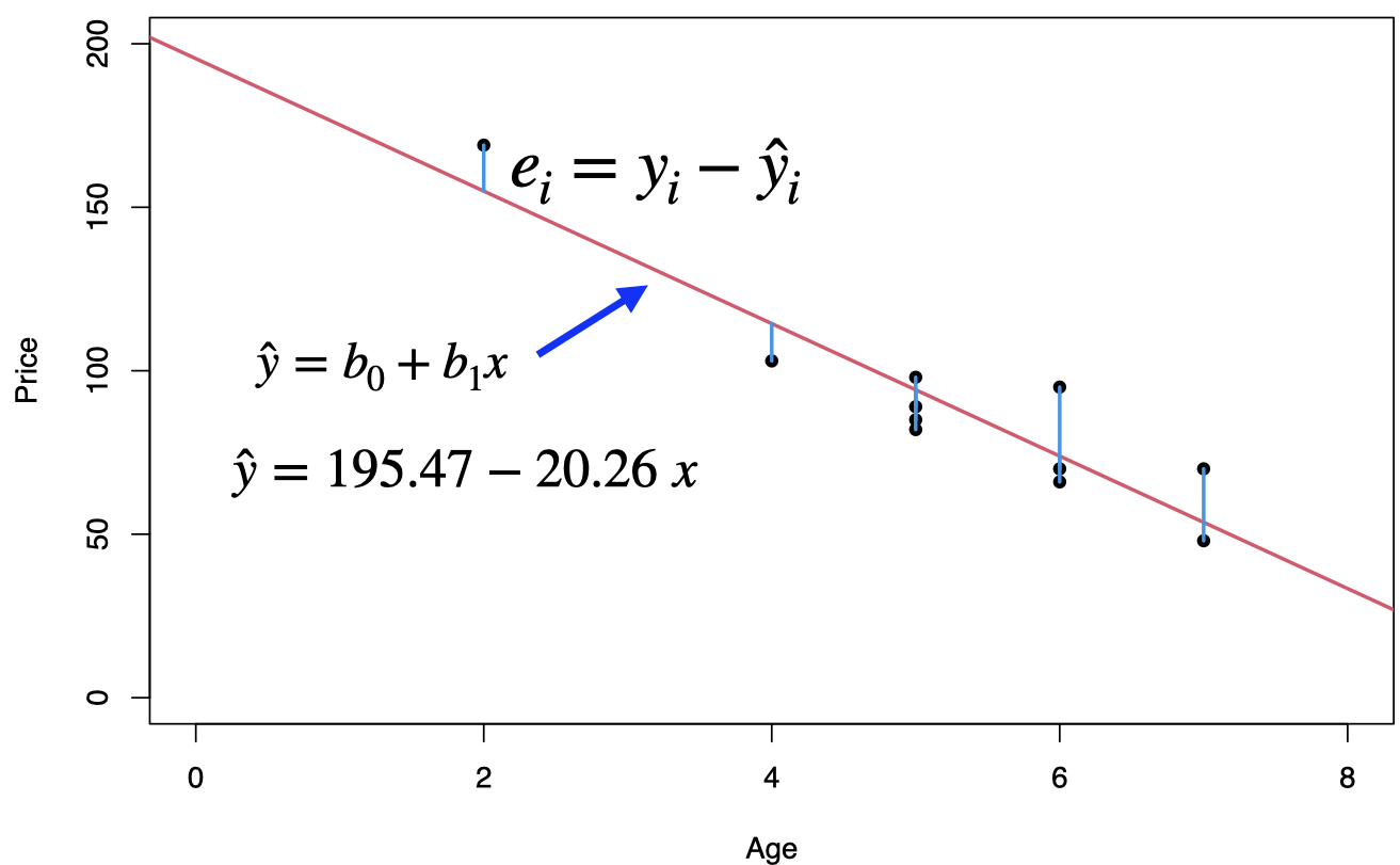
##      195.47       -20.26

To predict the price of a 4-year-old car ($x=4$): \[\hat{y}=195.47-20.26(4)=114.43\]

3 Simple Regression: Coefficient of Determination

3.1 Used cars example

The table below displays data on Age (in years) and Price (in hundreds of dollars) for a sample of cars of a particular make and model.(Weiss, 2012)

Price ($y$)	Age ($x$)
85	5
103	4
70	6
82	5
89	5
98	5
66	6
95	6
169	2
70	7
48	7

For our example, age is the predictor variable and price is the response variable.
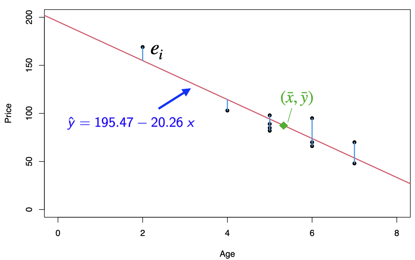
The regression equation is $\hat{y}=195.47-20.26\;x$, where the slope $b_1=-20.26$ and the intercept $b_0=195.47$
Prediction: for $x = 4$, that is we would like to predict the price of a 4-year-old car, \[\hat{y}=195.47-20.26 {\color{blue}(4)}= 114.43 \;\;\text{or}\;\; \$ 11443\]

3.2 Extrapolation

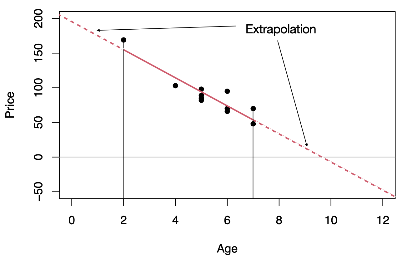
Within the range of the observed values of the predictor variable, we can reasonably use the regression equation to make predictions for the response variable.
However, to do so outside the range, which is called Extrapolation, may not be reasonable because the linear relationship between the predictor and response variables may not hold here.
To predict the price of an 11-year old car, $\hat{y}=195.47-20.26 (11)=-27.39$ or $ 2739, this result is unrealistic as no one is going to pay us $2739 to take away their 11-year old car.

3.3 Outliers and influential observations

Recall that an outlier is an observation that lies outside the overall pattern of the data. In the context of regression, an outlier is a data point that lies far from the regression line, relative to the other data points.
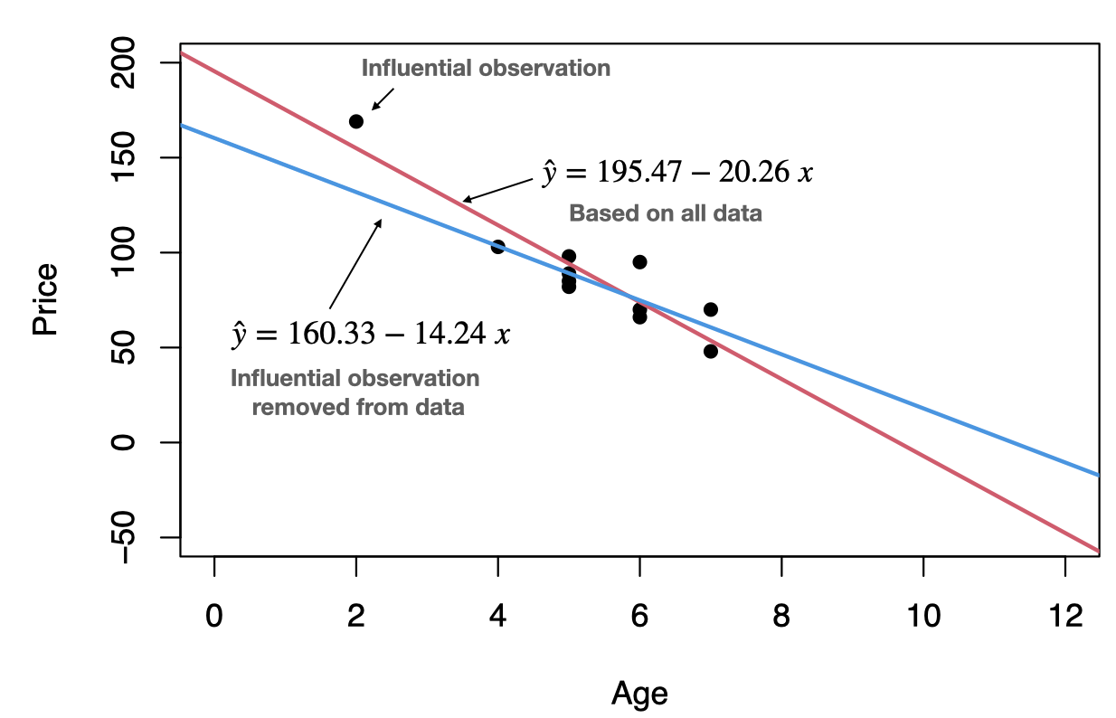
An influential observation is a data point whose removal causes the regression equation (and line) to change considerably.
From the scatterplot, it seems that the data point (2,169) might be an influential observation. Removing that data point and recalculating the regression equation yields $\hat{y}=160.33-14.24\;x$.

3.4 Coefficient of determination

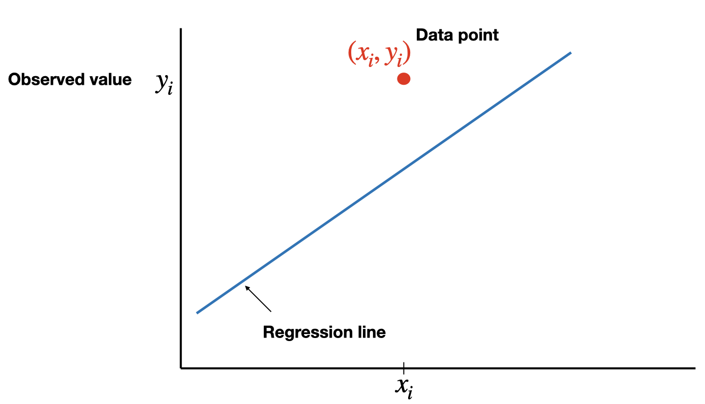
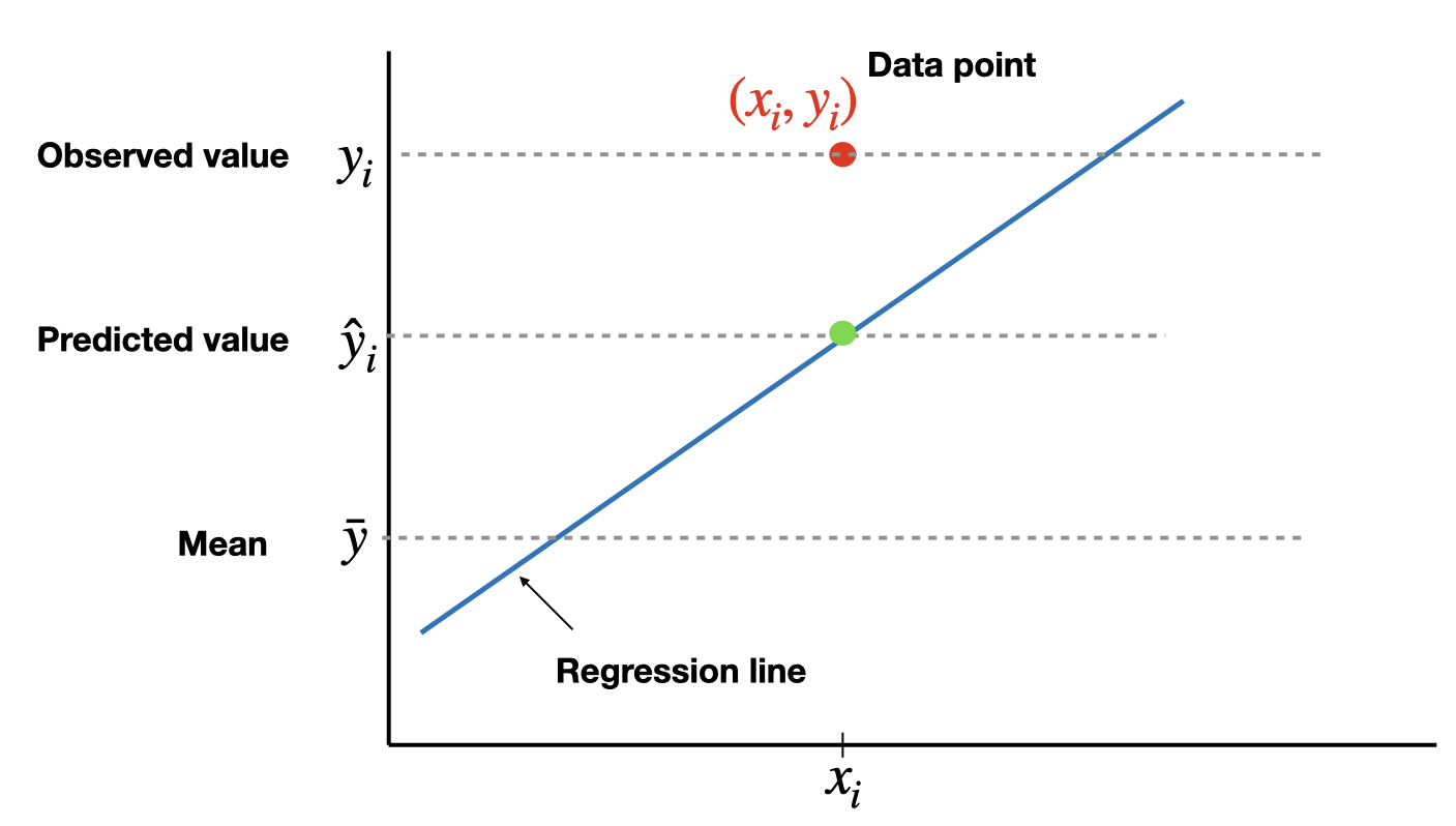
The total variation in the observed values of the response variable, $SST=\sum(y_i-\bar{y})^2$, can be partitioned into two components:
- The variation in the observed values of the response variable explained by the regression: $SSR=\sum(\hat{y}_i-\bar{y})^2$
- The variation in the observed values of the response variable not explained by the regression: $SSE=\sum(y_i-\hat{y}_i)^2$
The coefficient of determination, $R^2$ (or $R$-square), is the proportion of the variation in the observed values of the response variable explained by the regression, which is given by \[R^2=\frac{SSR}{SST}=\frac{SST-SSE}{SST}=1-\frac{SSE}{SST}\] where $SST=SSR+SSE$. $R^2$ is a descriptive measure of the utility of the regression equation for making prediction.
The coefficient of determination $R^2$ always lies between 0 and 1. A value of $R^2$ near 0 suggests that the regression equation is not very useful for making predictions, whereas a value of $R^2$ near 1 suggests that the regression equation is quite useful for making predictions.
For a simple linear regression (one independent variable) ONLY, $R^2$ is the square of Pearson correlation coefficient, $r$.
$\text{Adjusted}\;R^2$ is a modification of $R^2$ which takes into account the number of independent variables, say $k$. In a simple linear regression $k=1$. Adjusted-$R^2$ increases only when a significant related independent variable is added to the model. Adjusted-$R^2$ has a crucial role in the process of model building. Adjusted-$R^2$ is given by \[\text{Adjusted-}R^2=1-(1-R^2)\frac{n-1}{n-k-1}\]

3.5 Notation used in regression

Quantity	Defining formula	Computing formula
$S_{xx}$	$\sum (x_i-\bar{x})^2$	$\sum x^2_i - n \bar{x}^2$
$S_{xy}$	$\sum (x_i-\bar{x})(y_i-\bar{y})$	$\sum x_i y_i - n \bar{x}\bar{y}$
$S_{yy}$	$\sum (y_i-\bar{y})^2$	$\sum y^2_i - n \bar{y}^2$

where $\bar{x}=\frac{\sum x_i}{n}$ and $\bar{y}=\frac{\sum y_i}{n}$. And,

\[SST=S_{yy},\;\;\; SSR=\frac{S^2_{xy}}{S_{xx}},\;\;\; SSE=S_{yy}-\frac{S^2_{xy}}{S_{xx}} \] and $SST=SSR+SSE$.

Quantity	Defining formula	Computing formula
\(S_{xx}\)	\(\sum (x_i-\bar{x})^2\)	\(\sum x^2_i - n \bar{x}^2\)
\(S_{xy}\)	\(\sum (x_i-\bar{x})(y_i-\bar{y})\)	\(\sum x_i y_i - n \bar{x}\bar{y}\)
\(S_{yy}\)	\(\sum (y_i-\bar{y})^2\)	\(\sum y^2_i - n \bar{y}^2\)

Lecture 3