Workshop 4
In this workshop, we illustrate both parametric and non-parametric techniques for comparing two samples. Our objective in this workshop will be to assess whether or not two samples can be regarded as being from the same population. We perform the parametric version first, which requires normality assumptions of the data, and then move on to the non-parametric form which requires no normality assumptions.
To start, create a new R script by clicking on the corresponding menu button (in the top left); and save it somewhere in your computer. You can now write all your code into this file, and then execute it in R using the menu button Run or by simple pressing ctrl \(+\) enter.
\(~\)
1 The data
Eriksen, Björnstad an Götestam (1986) studied a social skills training program for alcoholics. Twenty-three alcohol-dependent male inpatients at an alcohol treatment centre were randomly assigned to two groups. The 12 control group patients were given a traditional treatment programme. The 11 treatment group patients were given the traditional treatment, plus a class in social skills training (“SST”). The patients were monitored for one year at 2-week intervals, and their total alcohol intake over the year was recorded (in cl pure alcohol).
| A: Control | 1042 | 1617 | 1180 | 973 | 1552 | 1251 | 1151 | 1511 | 728 | 1079 | 951 | 1391 |
| B: SST | 874 | 389 | 612 | 798 | 1152 | 893 | 541 | 741 | 1064 | 862 | 213 |
- Use the
cfunction to enter these data into R as two vectors calledAfor the control group, andBfor the treatment group. - Create summary statistics for both groups.
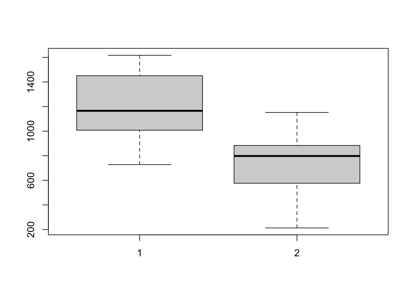
- Compare the distributions of
AandBusing a side-by-sideboxplot. What conclusions can you draw about the two groups? - Draw histograms (
hist) of both samples. On the basis of these plots, do the samples look approximately Normally distributed?
Click for solution
## SOLUTION
# (a)
A <- c(1042, 1617, 1180,  973, 1552, 1251, 1151, 1511,  728, 1079,  951, 1391)
B <- c(874,  389,  612,  798, 1152,  893,  541,  741, 1064,  862,  213)

# (b)
summary(A)
## Min. 1st Qu. Median Mean 3rd Qu. Max.
## 728 1025 1166 1202 1421 1617summary(B)## Min. 1st Qu. Median Mean 3rd Qu. Max.
## 213.0 576.5 798.0 739.9 883.5 1152.0# (c)
boxplot(A,B)
# (d)
par(mfrow=c(1,2))
hist(A)
hist(B)
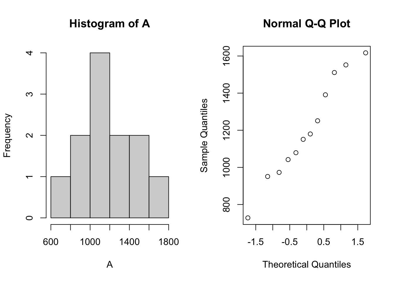
A better graphical way to assess whether the data is distributed normally is to draw a normal quantile plot (or quantile-quantile, or QQ plot). We can do this in R using the qqnorm function, where to draw the Normal quantile plot for a vector of data x we use the command
qqnorm(x)
With this technique, the quantiles of the data (i.e. the ordered data values) are plotted against the quantiles which would be expected of a matching normal distribution of a normal distribution. If the data are normally distributed, then the points of the QQ plot will should lie on an approximately straight line. Deviations from a straight line suggest departures from the normal distribution.
- Draw Normal quantile plots of both samples using
qqnorm. Do the samples look approximately Normally distributed? Do your conclusions agree with those made on the basis of the histograms? - Use Kolmogorov-Smirnov test and Shapiro-Wilk test to check the normality assumption of both samples. Do your conclusions agree with those made on the basis of the Normal quantile plots and the histograms?
Click for solution
## SOLUTION
# (a)
par(mfrow=c(1,2))
hist(A)
qqnorm(A)
par(mfrow=c(1,2))
hist(B)
qqnorm(B)
# Kolmogorov-Smirnov test
ks.test(A,"pnorm", mean=mean(A), sd=sd(A))
##
## One-sample Kolmogorov-Smirnov test
##
## data: A
## D = 0.12213, p-value = 0.9842
## alternative hypothesis: two-sidedks.test(B,"pnorm", mean=mean(B), sd=sd(B))##
## One-sample Kolmogorov-Smirnov test
##
## data: B
## D = 0.13791, p-value = 0.9666
## alternative hypothesis: two-sided# Shapiro-Wilk test
shapiro.test(A) ##
## Shapiro-Wilk normality test
##
## data: A
## W = 0.96414, p-value = 0.8409shapiro.test(B) ##
## Shapiro-Wilk normality test
##
## data: B
## W = 0.96798, p-value = 0.8654# Since all p-values are large, we do not reject the null hypothesis that
# the data are normally distributed.\(~\)
2 Two independent sample \(t\)-test
We will use the independent sample \(t\)-test to compare the two samples (ref to Lecture 2).
The t.test function, from the stats package, produces a variety of t-tests. Unlike most statistical packages, the default assumes unequal variance of the two samples, however we can override this with the var.equal argument.
# independent 2-sample t-test assuming equal variances and a pooled variance estimate
t.test(x,y,var.equal=TRUE)
# independent 2-sample t-test unequal variance and the Welsh df modification.
t.test(x,y)
t.test(x,y,var.equal=FALSE)You can use the alternative="less" or alternative="greater" options to specify a one-sided test.
A paired-sample \(t\)-test is obtained from the same function by specifying paired=TRUE and ensuring both samples are the same size:
# paired t-test
t.test(x,y,paired=TRUE)
Finally, a one-sample \(t\)-test can be performed to test the population mean \(\mu\) of the sample against a specific value by supplying only a single sample and a value for mu:
# one sample t-test
t.test(y,mu=3) # Ho: mu=3
R Help: t.test
\(~\)
- Use the function
t.testto compare these two samplesAandB. Use the optional argumentvar.equalto perform an equal-variance test (TRUE). - Extract the t statistic value from the output summary from R, and save it as
t. - Perform the significance test: test \(H_0: \mu_A=\mu_B\) against \(H_1: \mu_A\neq\mu_B\) at the 5% level of significance.
- Obtain a 95% confidence interval for the difference in means between the two populations.
Click for solution
# (a)
library(stats)
t.test(A,B, alternative = "two.sided", var.equal=TRUE)
##
## Two Sample t-test
##
## data: A and B
## t = 4.0076, df = 21, p-value = 0.0006381
## alternative hypothesis: true difference in means is not equal to 0
## 95 percent confidence interval:
## 222.3822 702.1329
## sample estimates:
## mean of x mean of y
## 1202.1667 739.9091# (b)
t<-t.test(A,B, alternative = "two.sided", var.equal=TRUE)$statistic
t## t
## 4.00757# (c) we can also extract the p-value from the output summary
p<-t.test(A,B, alternative = "two.sided", var.equal=TRUE)$p.value
p #Since the p-value is less than 0.05 we reject H0## [1] 0.0006380701# (d)
t.test(A,B, alternative = "two.sided", var.equal=TRUE, conf.level = 0.95)$conf.int## [1] 222.3822 702.1329
## attr(,"conf.level")
## [1] 0.95\(~\)
We can also perform the significance test by comparing the value of the \(t\) test statistic to the critical value.
- How many degrees of freedom do we associate with the distribution of \(t\)? Save this value to a variable
df - How would you use the
[qt](r_5_basicstats.html#dist) function to find the critical \(t\) value for the test of \(H_0: \mu_A=\mu_B\) against \(H_1: \mu_A\neq\mu_B\) at the 5% level of significance when we havedfdegrees of freedom? Check you get the same value as below.
Click for solution
# (a)
n <- length(A)
m <- length(B)
df <- n+m-2
df
## [1] 21# (b)
tcrit <- qt(0.975, df=df)
tcrit## [1] 2.079614\(~\)
- Compare this to your value of
t, and hence perform the significance test. - What is the probability of observing a value of the test statistic whose absolute value is at least as large as the one observed under the null hypothesis? i.e. what is \(P[T_{df}\geq t]\)
- On the basis of your calculations above, what would you conclude about the population means for the two groups \(A\) and \(B\)?
- Do you think the assumption of equal variances holds here? If not, would this affect your conclusions?
Click for solution
# (a)
t<-t.test(A,B, alternative = "two.sided", var.equal=TRUE)$statistic
t
## t
## 4.00757t<-unname(t)
t## [1] 4.00757tcrit <- qt(0.975, df=df)
tcrit## [1] 2.079614# Since the absolute value of the test statistic is greater than the critical value, $t_{1-\alpha/2},df$, tcrit, we reject H0.
# (b)
pvalue <- 2*(1-pt(t,df))
pvalue## [1] 0.0006380701# (c)
# Strong evidence here to reject H_0 at 5% level, sample sizes are rather small
# (d)
# From the boxplots, this assumption does not look unreasonable though perhaps B is slightly less spread than A.\(~\)
- Apply the independent sample \(t\)-test with unequal variances to compare the two groups. Use the function
t.testand the optional argumentvar.equal=FALSEto perform an unequal-variance test. - What do you conclude? Do the results agree with or contradict the equal-variance test?
Click for solution
# (a)
t.test(A,B, alternative = "two.sided", var.equal=FALSE)
##
## Welch Two Sample t-test
##
## data: A and B
## t = 4.0013, df = 20.674, p-value = 0.0006644
## alternative hypothesis: true difference in means is not equal to 0
## 95 percent confidence interval:
## 221.7733 702.7418
## sample estimates:
## mean of x mean of y
## 1202.1667 739.9091# (b)
## Results don't change much, looks like the equal-variance assumption was safe\(~\)
3 Nonparametric rank-sum test
Nonparametric methods do not assume any distribution, and try to make only the weakest possible assumptions about the distributions that describe our data and are often used in such situations. The nonparametric equivalent to the independent sample \(t\)-test is the (Wilcoxon) rank-sum test. Nonparametric tests do not assume knowledge of the distributions of the two groups, and are often based on the data ranks with tests comparing the data ranks of the two groups.
3.1 The rank-sum test
Recall that the rank-sum test statistic is the sum of the ranks of the first sample (of size \(n\)) in the combined sample (of size \(n+m\) where \(m\) is the size of the second sample), that is \[ W = \sum_{i=1}^n r_i. \]
The exact critical value for the rank-sum test \(W\) is a function of the sample sizes, \(n\) and \(m\), and the significance level, \(\alpha\) (see the statistical tables on Ultra). When the samples are both large, the distribution of the rank-sum statistic is approximately Normal, which allows us to use Normal tables to construct confidence intervals and test hypotheses.
Note: the reported value of the rank-sum test statistic using the R function wilcox.test is \(W-\frac{n(n+1)}{2}\).
- Use the
cfunction to combine the two samples together into a larger vector composed of the elements of the A group followed by the B group. - Use the
rankfunction on the combined sample to rank all the observations; call thisrks. - The first \(n\) elements of
rksshould now be the ranks \(r_i\) for the A group in the combined sample. Extract these from the larger vector and save them asAranks. - Find the rank-sum test statistic for the A group.
- Read the help for the
wilcox.testfunction function and try it onAandB. The optional argumentexact=TRUEwill compute the test exactly, whereasexact=FALSEwill use a Normal approximation. Do the results agree with your t-test results?
Click for solution
# (a)
AB <- c(A,B)

# (b)
rks <- rank(AB)

# (c)
## statistic for group A
Aranks <- rks[1:n]

# (d)
W <- sum(Aranks)
W
## [1] 195# (e)
wilcox.test(A,B,exact=TRUE)##
## Wilcoxon rank sum exact test
##
## data: A and B
## W = 117, p-value = 0.0009807
## alternative hypothesis: true location shift is not equal to 0wilcox.test(A,B,exact=TRUE)$statistic## W
## 117wilcox.test(A,B,exact=FALSE)##
## Wilcoxon rank sum test with continuity correction
##
## data: A and B
## W = 117, p-value = 0.001883
## alternative hypothesis: true location shift is not equal to 0wilcox.test(A,B,exact=FALSE)$statistic## W
## 117# we get the same value of the test statistic as in (d).
# since the p-values are less than 0.05 we reject H0,
# so we have the same conclusion as with the t-test.\(~\)