In this workshop, we will investigate the behaviour and distributions of summary statistics calculated from samples of normally-distributed data. To do this, we will use R to simulate large numbers of Normal random samples, and from each of which we will compute the sample mean and variance. By repeating this experiment for a large number of such samples, we will accumulate a large number of sample means and variances which we will investigate and compare to the results we would expect to find from the theory in lectures.

To start, create a new R script by clicking on the corresponding menu button (in the top left); and save it somewhere in your computer. You can now write all your code into this file, and then execute it in R using the menu button Run or by simple pressing ctrl \(+\) enter.

1 Normal Sampling Theory

First, let’s recap a little theory. Consider a sample of \(n\) Normally-distributed data points: \(X_1,\dots,X_n\) i.i.d random variables from \(N(\mu,\sigma^2)\). We can say:

The sample mean \(\bar{X}\) has distribution:

\[ \bar{X} = \frac{1}{n} \sum_{i=1}^n X_i \sim N \left( \mu,\frac{\sigma^2}{n} \right).\]

The sample variance \(S^2\) is independent of \(\bar{X}\), and is such that

\[ \frac{(n-1)}{\sigma^2} S^2 \sim \chi^2_{n-1}.\]

If we standardise \(\bar{X}\) using the sample standard deviation \(S\) instead of the population standard deviation \(\sigma\), we don’t get a Normal distribution - we get the following \(t\) distribution instead:

\[T=\frac{\bar{X}-\mu}{S/\sqrt{n}} \sim t_{n-1}.\]

2 Generating the samples

In order to illustrate this theory, we require a large number of samples from normal distributions that will act as our data in the following calculations. To generate the random numbers from a normal distribution, we will use the rnorm function.

We can use the rnorm function to generate random numbers from a normal distribution. To generate n random normal variates from a Normal distribution with mean m and standard deviation s, we use the command:

rnorm(n, mean=m, sd=s)

The mean and sd arguments are optional, and default to \(0\) and \(1\) respectively if missing.

For more details, see random number generation.

Use the rnorm function to try generating:
1. 5 random standard Normal numbers
2. 20 random numbers from \(N(5,5^2)\)
Check the mean and standard deviation of your sample using the mean and sd functions - are the values what you expected?

Click for solution

samp1 <- rnorm(5) ## 5 standard normals
mean(samp1) ## expect mean approx 0, but sample is small so we wouldn't worry if we weren't close

## [1] 0.5594011

var(samp1)  ## and var approx 1

## [1] 0.6503027

samp2 <- rnorm(20,mean=5,sd=5) ## set mean and sd arguments to get N(5,25)
mean(samp2) ## expect about 5

## [1] 7.40592

sd(samp2) ## expect sqrt(25)=5

## [1] 4.032326

\(~\)

Now we’re ready to construct our data set. Using rnorm, generate a vector of 500 random standard normal values, and save it to a variable zs. Check the mean and standard deviation are consistent with the population distribution.

Click for solution

zs <- rnorm(500)
zs[1:5] ## print the first few elements

## [1] -0.2829437  1.2558840  0.9098392 -0.9280281  1.2401808

mean(zs)

## [1] -0.06422456

sd(zs)

## [1] 0.9678852

\(~\)

Let’s change the mean and variance of our sample to make things (fractionally) more interesting. Let’s suppose we want our data to come from a normal population with mean 17 and standard deviation 5.

Recall that if \(Z \sim N(0,1)\), then \((a+bZ) \sim N(a,b^2)\) - use this result to apply the appropriate transformation to zs to correspond with the new population mean and variance, and save the result to a new variable xs.
Check the mean and standard deviation of xs to ensure your transformation worked as intended.
Hint: you can apply standard arithmetic to vectors in R.

Click for solution

xs <- 17+5*zs
xs[1:5]

## [1] 15.58528 23.27942 21.54920 12.35986 23.20090

mean(xs)

## [1] 16.67888

sd(xs)

## [1] 4.839426

\(~\)

Next, we want to treat our 500 \(X\) values as if they were 100 different random samples, each of size 5. To do this, we will transform our vector of length 500 into a matrix with 100 rows and 5 columns. This way, each of the rows in the matrix corresponds to a different random sample of size 5.

A matrix is created using the matrix function, which takes three arguments: the values of the matrix (data), the number of rows (nrow), and the number of columns (ncol).

To produce a \(3\times3\) matrix containing the integers 1 to 9, we would write:

matrix(1:9, nrow = 3, ncol=3)

For more details, see the techniques page on matrices.

Use the matrix function to create a \(100\times5\) matrix from the values in xs. Save the result as xMatrix.

Click for solution

xMatrix <- matrix(xs, nr=100, nc=5)
xMatrix[1:3,] ## print the first few rows

##          [,1]     [,2]      [,3]     [,4]      [,5]
## [1,] 15.58528 21.93914  9.807528 20.46792 14.167605
## [2,] 23.27942 12.29372 20.171829 12.00987 17.195204
## [3,] 21.54920 18.74593 14.504026 12.00182  7.444389

\(~\)

3 Investigating \(\bar{X}\)

To investigate the behaviour of \(\bar{X}\), we need some data. From the previous step, we have effectively generated 100 Normal samples each of size 5, each represented by a row in xMatrix. What we want to do now to calculate the sample mean for each of these samples (i.e every row). This will give us a collection of 100 observed sample mean values, \(\bar{x}\), drawn from the distribution of \(\bar{X}\) which we can investigate more closely.

Last time we saw how to use the sapply function to repeatedly apply a function to every element of a vector.

When we want to apply a function over a matrix, we use the apply function, which evaluates the same function to either every row or every column of a given matrix (or data frame). This is particularly useful for computing summary statistics (means, standard deviations, etc) for all variables in a data set.

The apply function takes three arguments:

X - the matrix or data frame to use for calculations
MARGIN - which indicates whether to evaluate over the rows (MARGIN=1) or columns (MARGIN=2) of the matrix
FUN - the name of the function we wish to evaluate.

For example, to calculate the minimum value in each column of a matrix A, we could write

apply(A, MARGIN=2, FUN=min)

For more details, see the techniques page on apply.

Use the apply function to compute the sample mean for every row of xMatrix. You should obtain a vector of length 100. Save the results as xbar.
Calculate the mean and variance of xbar - do they agree with the values that we would expect from the theoretical distribution of \(\bar{X}\) given above?

Click for solution

xbar <- apply(xMatrix, MARGIN=1, FUN=mean)
xbar[1:5]

## [1] 16.39350 16.99001 14.84907 16.21545 17.48049

\(~\)

Now we’ll use the hist function to plot a histogram of the xbar values from our sample, and we’ll overlay the Normal density curve we’d expect from the theory on top of the histogram using lines.

If you’re unfamiliar with plotting histograms with hist, quickly read up on the hist function.
Use hist to draw a histogram of xbar setting breaks=15 to ensure we show enough detail in the bars in the plot, and set freq=FALSE to plot the vertical axis as frequency density instead of frequency.

Click for solution

hist(xbar,freq=FALSE,breaks=15)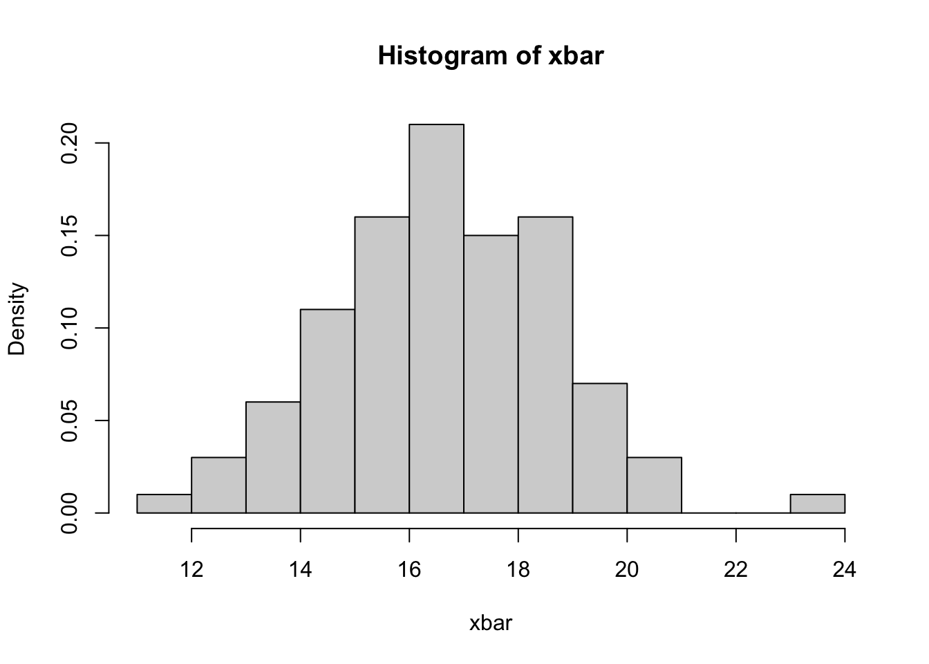

\(~\)

To produce the Normal density curve on top of the histogram, we need to evaluate the pdf of \(\mathcal{N}\left({\mu, \sigma^2/n}\right)\) over the plotting range of the histogram, and then use lines to draw the function on top.

R provides a range of functions to support calculations with standard probability distributions. To save creating our own functions to evaluate the pdfs and cdfs, we can use these standard functions instead.

For every distribution there are four functions. The functions for each distribution begin with a particular letter to indicate the functionality (see table below) followed by the name of the distribution:

Letter	e.g.	Function
“d”	`dnorm`	evaluates the probability density (or mass) function, \(f(x)\)
“p”	`pnorm`	evaluates the cumulative density function, \(F(x)=P[X \leq x]\), hence finds the probability the specified random variable is less than the given argument.
“q”	`qnorm`	evaluates the inverse cumulative density function (quantiles), \(F^{-1}(q)\) i.e. given a probability \(q\) it returns the value \(x\) such that \(P[X \leq x] = q\). Used to obtain critical values associated with particular probabilities \(q\).
“r”	`rnorm`	generates random numbers

We’ve already seen one example with rnorm to generate random Normal values. The appropriate functions for Normal, \(t\) and \(\chi^2\) distributions are given below, along with the optional parameter arguments.

Normal distribution: dnorm, pnorm, qnorm, rnorm. Parameters: mean (\(\mu\)) and sd (\(\sigma\)).
\(t\) distribution: dt, pt, qt, rt. Parameter: df.
\(\chi^2\) distribution: dchisq, pchisq, qchisq, rchisq. Parameter: df.

For a list of all the supported distributions, run the command help(Distributions)

First, construct a sequence of values (using seq) which starts at the minimum of xbar and goes up to the maximum value of xbar and has length 100. Save this vector as seqx. Hint: You’ll need the seq, min, and max functions - see here for help if needed.
Use dnorm to evaluate the normal density function at the values seqx and save these values as ndens. Try this now. Make sure you supply the correct value of \(\mu\) to the mean argument, and \(\sigma/\sqrt{n}\) to the sd argument, otherwise your pdf won’t match the histogram.

Click for solution

seqx <- seq(min(xbar)-1, max(xbar)+1, length=100)
ndens <- dnorm(seqx, mean=17, sd=5/sqrt(5))

\(~\)

We can use R’s line drawing function lines to add an (approximate) curve to a plot. To draw a function \(f(x)\) on an existing plot, we evaluate the function \(f\) at a sequence of \(x\) points and then use lines to draw connected line segments between each \((x,f(x))\) pair to form the curve.

For example, if we save the \(x\) values in a vector xs and the \(~f(x)\) values in a vector fs then the command to add the curve to the plot is:

lines(x=xs, y=fs)

Like other plotting functions, lines can be modified by adding argumets to specify different line types and colours for your curve.

Use the lines function to add a solid blue curve between the points x=seqx and y=ndens to your histogram.
How does the distribution of our sample of \(\bar{x}\) values compare (in terms of shape, location, and spread) with the theoretical distribution of \(\bar{X}\)? Does it agree with the theory?

Click for solution

hist(xbar,freq=FALSE,breaks=15)
seqx <- seq(min(xbar)-1, max(xbar)+1, length=100)
ndens <- dnorm(seqx, mean=17, sd=5/sqrt(5))
lines(x=seqx, y=ndens, col='blue')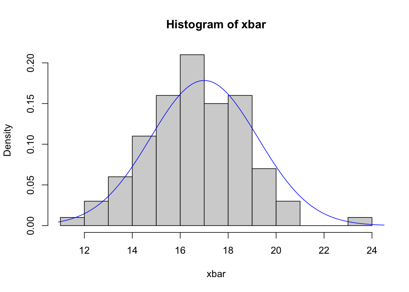

\(~\)

Note: if your density curve goes off the top of your plot, then try redrawing the histogram but set the limits of the vertical axis by passing the ylim=c(a,b) argument to the hist function where a and b are your desired upper and lower limits of the \(y\) axis. Use a lower limit of 0 and choose the upper limit to be large enough to see the entire curve.

4 Investigating \(S^2\) and \(T\)

Now let’s move on to investigate the sample variances and standardised values. If our data are normal, then a multiple of the sample variance, namely \(\frac{n-1}{\sigma^2}S^2\), should follow a \(\chi^2_{}\) distribution with \(n-1\) degrees of freedom. Let’s compute the sample variances for our 100 samples and investigate this using the techniques above.

Apply the var function to each of the samples in xMatrix to create a vector of 100 sample variances, \(s^2\). Call these svar.
The theory says that the random quantity \(\frac{n-1}{\sigma^2}S^2\) has a \(\chi^2_{n-1}\) distribution. Re-scale the sample variances by multiplying svar by \(\frac{n-1}{\sigma^2}\), and call this svarScl (for ‘scaled sample variance’).
Calculate the mean and variance of svarScl - do they agree with the mean and variance of the appropriate \(\chi^2_{n-1}\) distribution?
By modifying your code from Ex 3.2-3.4, plot a histogram of \(s^2\) and overlay the density function for a \(\chi^2_{n-1}\) distribution using the dchisq function. Do the samples appear consistent with the theoretical distribution?
According to the theory, \(\bar{X}\) and \(S^2\) should be independent. Use plot to produce a scatterplot of \(\bar{x}\) against \(s^2\). Do they appear to be independent? What features of the plot support this conclusion?

Click for solution

# (a)
svar <- apply(xMatrix, MARGIN=1, FUN=var)

# (b)
svarScl <- (5-1)/5^2 * svar

# (c)
mean(svarScl) ## expect mean = df = (n-1) = 4

## [1] 3.81259

var(svarScl)  ## expect var = 2*df = 2*(n-1) = 8

## [1] 7.005375

# (d)
hist(svarScl,freq=FALSE,breaks=15,ylim=c(0,0.2))
tmpx <- seq(0, max(svarScl), length=100)
chisqdens <- dchisq(tmpx, df=(5-1))
lines(x=tmpx, y=chisqdens, col='red', lwd=2)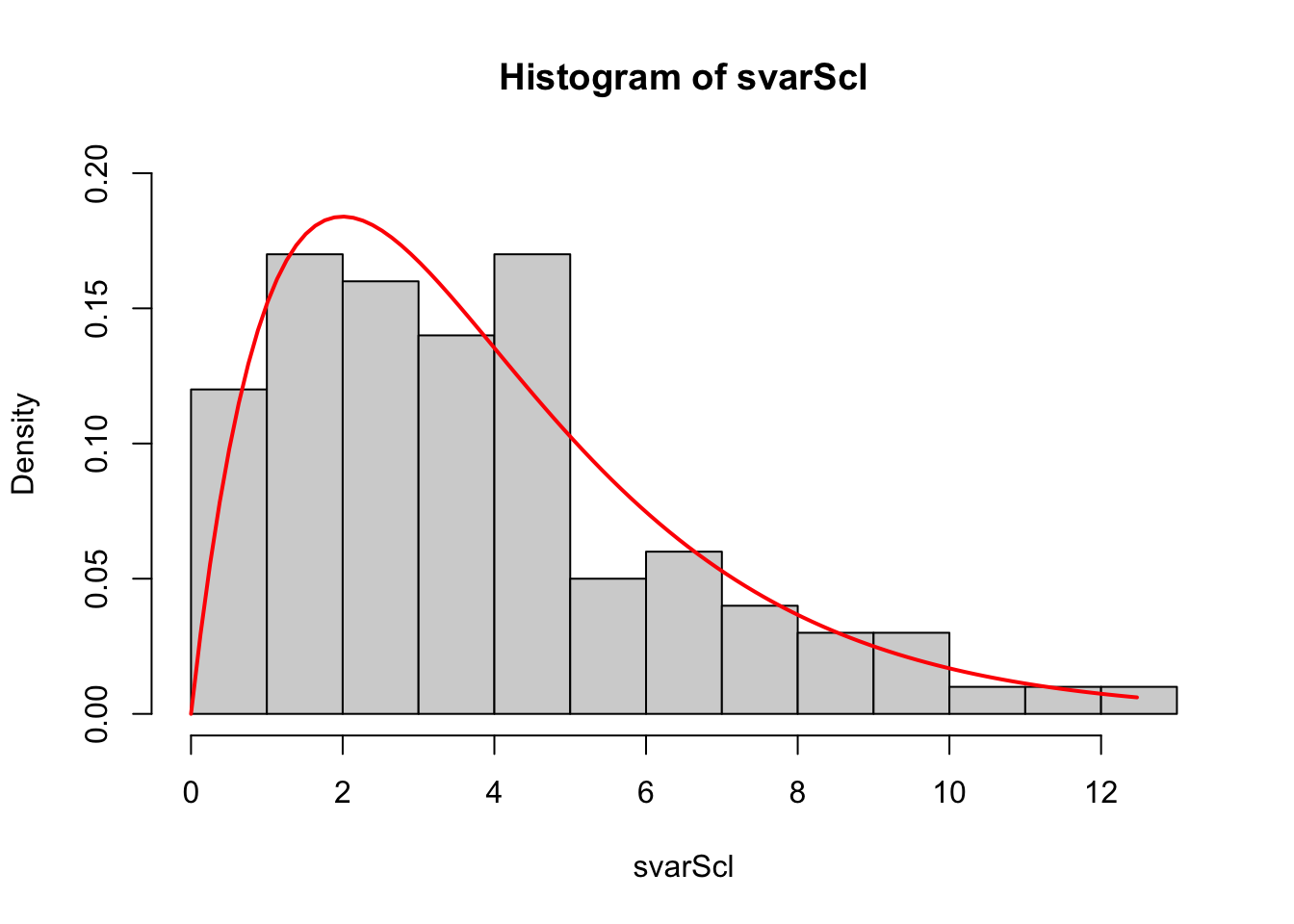

# (e)
plot(x=xbar, y=svar) ## we expect to see unstructured random scatter with no pattern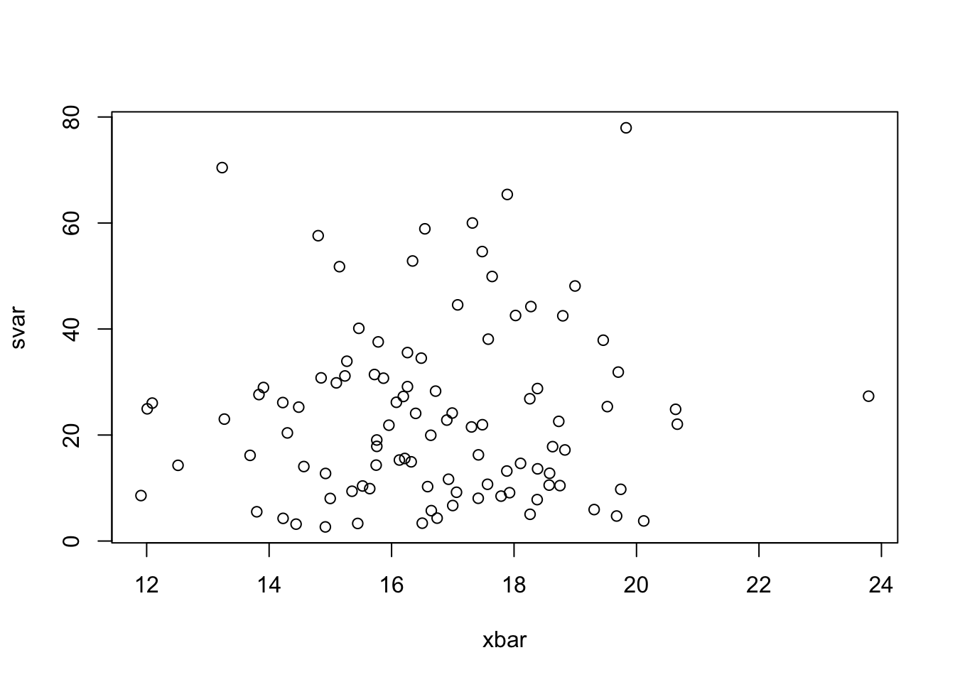

\(~\)

The final result concerns the distribution of the sample means when standardised by the sample variance, \(T=\frac{\bar{X}-\mu}{s/\sqrt{n}}\). We know that if we use the population variance, \(\sigma^2\), in this calculation instead of \(s^2\), then the standardised values are \(\mathcal{N}\left({0,1}\right)\). However, as this expression uses the sample variance the distribution is no longer normal, and is \(t\)-distributed instead to account for the extra uncetainty we have introduced by using an estimate of \(\sigma^2\).

Using your values of xbar and svar, create a new vector tvals with elements equal to \(\frac{\bar{x}-\mu}{s/\sqrt{n}}\) for each sample of size 5.
Using the techniques above, investigate the behaviour and distribution of tvals (inspect the mean and variance, construct a histogram, overlay the appropriate density curve).

Click for solution

# (a)
tvals <- (xbar-17)/sqrt(svar/5)
mean(tvals) ## expect mean=0

## [1] -0.1986574

var(tvals)  ## expect var=df/(df-2)

## [1] 1.623998

# (b)
hist(tvals,freq=FALSE,breaks=15)
tmpx <- seq(min(tvals), max(tvals), length=100)
tdens <- dt(tmpx, df=(5-1))
lines(x=tmpx, y=tdens, col='red', lwd=2)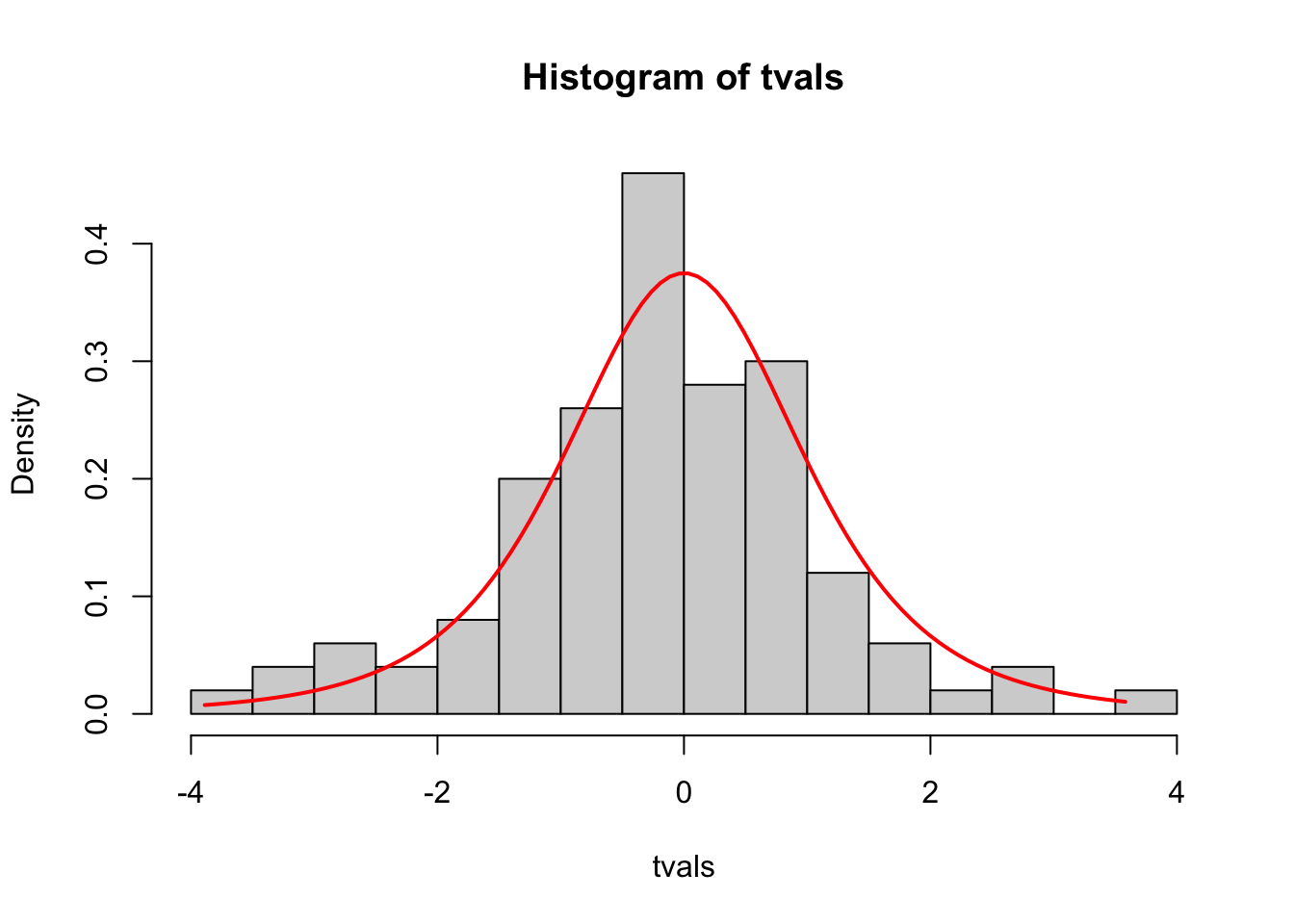

\(~\)

Workshop 3

1 Normal Sampling Theory

2 Generating the samples

3 Investigating \(\bar{X}\)

4 Investigating \(S^2\) and \(T\)