Lecture 1
1 Install R and RStudio
In this course, we will learn how to use R and RStudio for data analysis and visualization. Before we do that you will need to install R and RStudio locally on your computer. Both are free to download from the links below. Please notice that you need to download R first then RStudio.
Both R and RStudio are also available on the University network via AppsAnywhere.
https://appsanywhere.durham.ac.uk/
Watch the video for a step-by-step instructions on how to install R and RStudio on your computer.
2 Basic Concepts
2.1 Some basic concepts
Data consist of information coming from observations, counts, measurements, or responses.
Statistics is the science of collecting, organizing, analyzing, and interpreting data in order to make decisions.
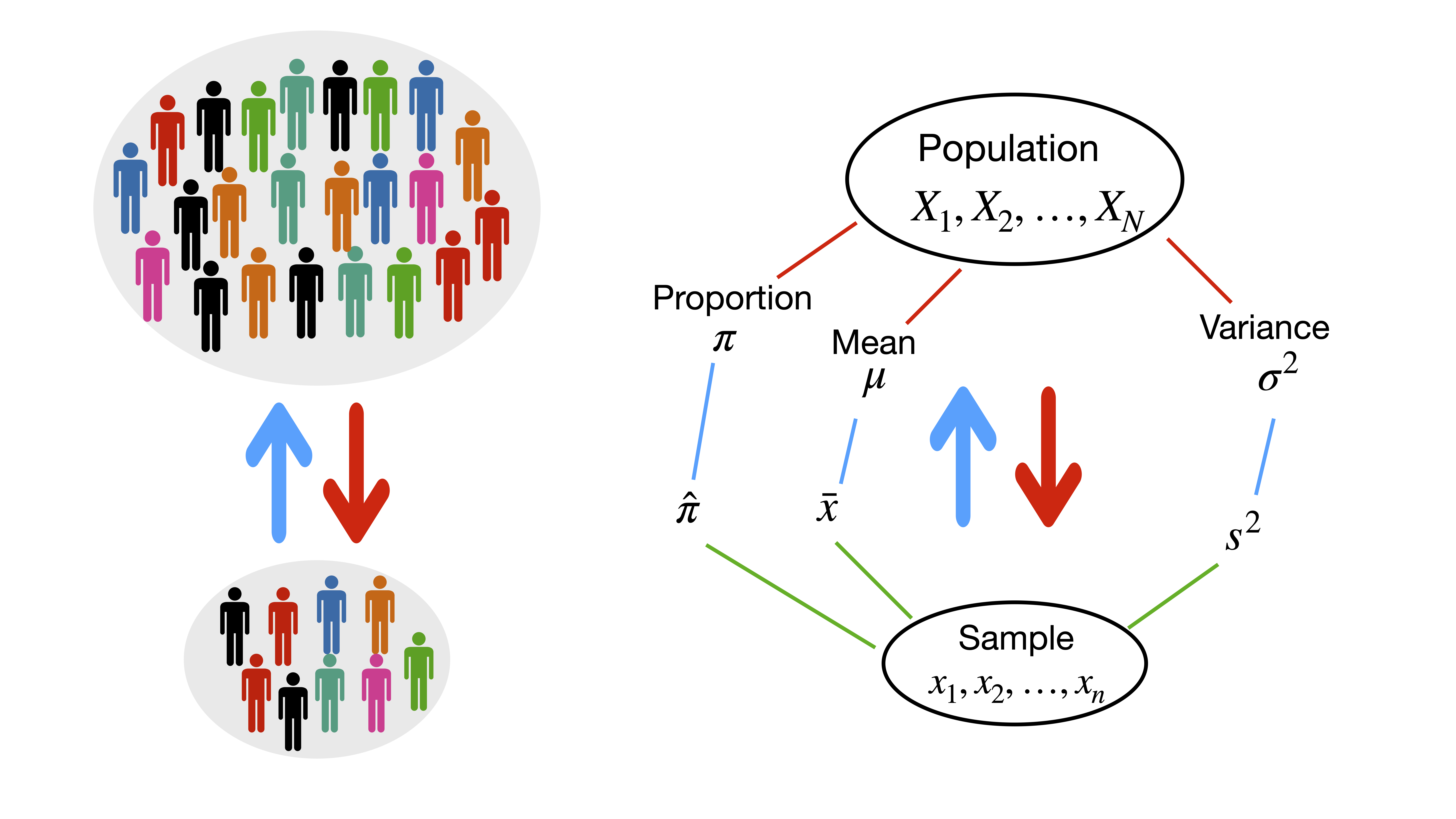
A population is the collection of all outcomes, responses, measurements, or counts that are of interest. Populations may be finite or infinite. If a population of values consists of a fixed number of these values, the population is said to be finite. If, on the other hand, a population consists of an endless succession of values, the population is an infinite one.
A sample is a subset of a population.
A parameter is a numerical description of a population characteristic.
A statistic is a numerical description of a sample characteristic.
2.2 Branches of statistics
The study of statistics has two major branches - descriptive statistics and inferential statistics:
Descriptive statistics is the branch of statistics that involves the organization, summarization, and display of data.
Inferential statistics is the branch of statistics that involves using a sample to draw conclusions about a population, e.g. estimation and hypothesis testing.
2.3 What is the idea?
2.4 Notation
| Population | Sample | |
|---|---|---|
| Size | \(N\) | \(n\) |
| Parameter | Statistic | |
| Mean | \(\mu\) | \(\bar{x}\) |
| Variance | \(\sigma^2\) | \(s^2\) |
| Standard deviation | \(\sigma\) | \(s\) |
| Proportion | \(\pi\) | \(\hat{\pi}\) |
| Correlation | \(\rho\) | \(r\) |
3 Data Types in Statistics
3.1 Data collection methods (Traditional data)
There are several ways for collecting data:
- Take a census: a census is a count or measure of an entire population. Taking a census provides complete information, but it is often costly and difficult to perform.
- Use sampling: a sample is a count or measure of a part of a population. Statistics calculated from a sample are used to estimate population parameters.
- Use a simulation: collecting data often involves the use of computers. Simulations allow studying situations that are impractical or even dangerous to create in real life and often save time and money.
- Perform an experiment: e.g. to test the effect of imposing a new marketing strategy, one could perform an experiment by using the new marketing strategy in a certain region.
3.2 Data collection methods (Big data)
The characteristics of big data (the 4Vs?):
- Volume: how much data is there?
- Variety: different types of data?
- Velocity: at what speed?
- Veracity: how accurate?
3.3 Types of data
Data sets can consist of two types of data:
Qualitative (categorical) data consist of attributes, labels, or nonnumerical entries. e.g. name of cities, gender etc.
Quantitative data consist of numerical measurements or counts. e.g. heights, weights, age. Quantitative data can be distinguished as:
Discrete data result when the number of possible values is either a finite number or a “countable” number. e.g. the number of phone calls you received in any given day.
Continuous data result from infinitely many possible values that correspond to some continuous scale that covers a range of values without gaps, interruptions, or jumps. e.g. height, weight, sales and market shares.
3.4 Types of data (Econometrics)
Cross-sectional data: Data on different entities (e.g. workers, consumers, firms, governmental units) for a single time period. For example, data on test scores in different school districts.
Time series data: Data for a single entity (e.g. person, firm, country) collected at multiple time periods. For example, the rate of inflation and unemployment for a country over the last 10 years.
Panel data: Data for multiple entities in which each entity is observed at two or more time periods. For example, the daily prices of a number of stocks over two years.
3.5 Levels of measurement
Nominal: Categories only, data cannot be arranged in an ordering scheme. (e.g. Marital status: single, married etc.)
Ordinal: Categories are ordered, but differences cannot be determined or they are meaningless (e.g. poor, average, good)
Interval: differences between values are meaningful, but there is no natural starting point, ratios are meaningless (e.g. we cannot say that the temperature 80\(^{\circ}\)F is twice as hot as 40\(^{\circ}\)F)
Ratio: Like interval level, but there is a natural zero starting point and rations are meaningful (e.g. is twice as much as )
4 Descriptive Statistics
4.1 Measures of Central Tendency
Measures of central tendency provide numerical information about a `typical’ observation in the data.
- The Mean (also called the average) of a data set is the sum of the data values divided by the number of observations.
\[\;\;\;\; \text{Sample mean:}\;\;\; \bar{x}=\frac{1}{n}\sum_{i=1}^{n}x_i\]
- The Median is the middle observation when the data set is sorted in ascending or descending order. If the data set has an even number of observations, the median is the mean of the two middle observations.
- The Mode is the data value that occurs with the greatest frequency. If no entry is repeated, the data set has no mode. If two (more than two) values occur with the same greatest frequency, each value is a mode and the data set is called bimodal (multimodal).
4.2 Measure of Variation (Dispersion)
The variation (dispersion) of a set of observations refers to the variability that they exhibit.
Range = maximum data value - minimum data value
The variance measures the variability or spread of the observations from the mean.
\[\text{Sample variance:}\;\;\;s^2=\frac{1}{n-1}\sum_{i=1}^{n}(x_i-\bar{x})^2\]
Shortcut formula for sample variance is given by \[\text{Sample variance:}\;\;\;s^2=\frac{1}{n-1}\left\{\sum_{i=1}^{n}x^2_i-n\bar{x}^2\right\}\]
The standard deviation (\(s\)) of a data set is the square root of the sample variance.
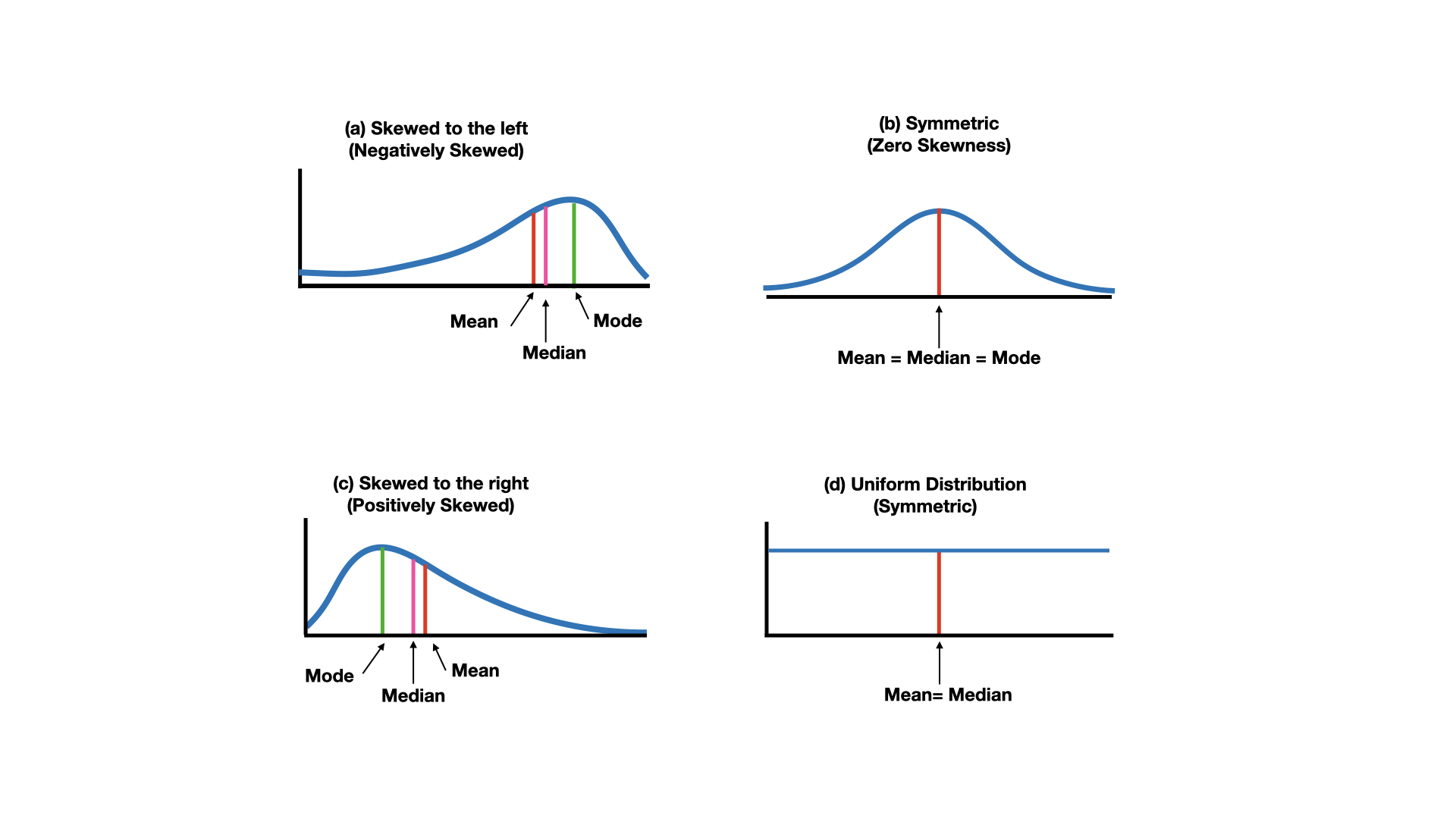
4.3 Shape of a distribution: Skewness
Skewness is a measure of the asymmetry of the distribution.
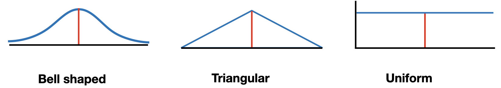
4.4 Shape of a distribution: Kurtosis
Kurtosis measures the degree of peakedness or flatness of the distribution.

4.5 Modality

4.6 Symmetry
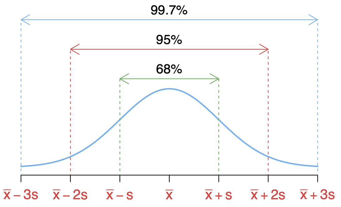
4.7 Empirical Rule
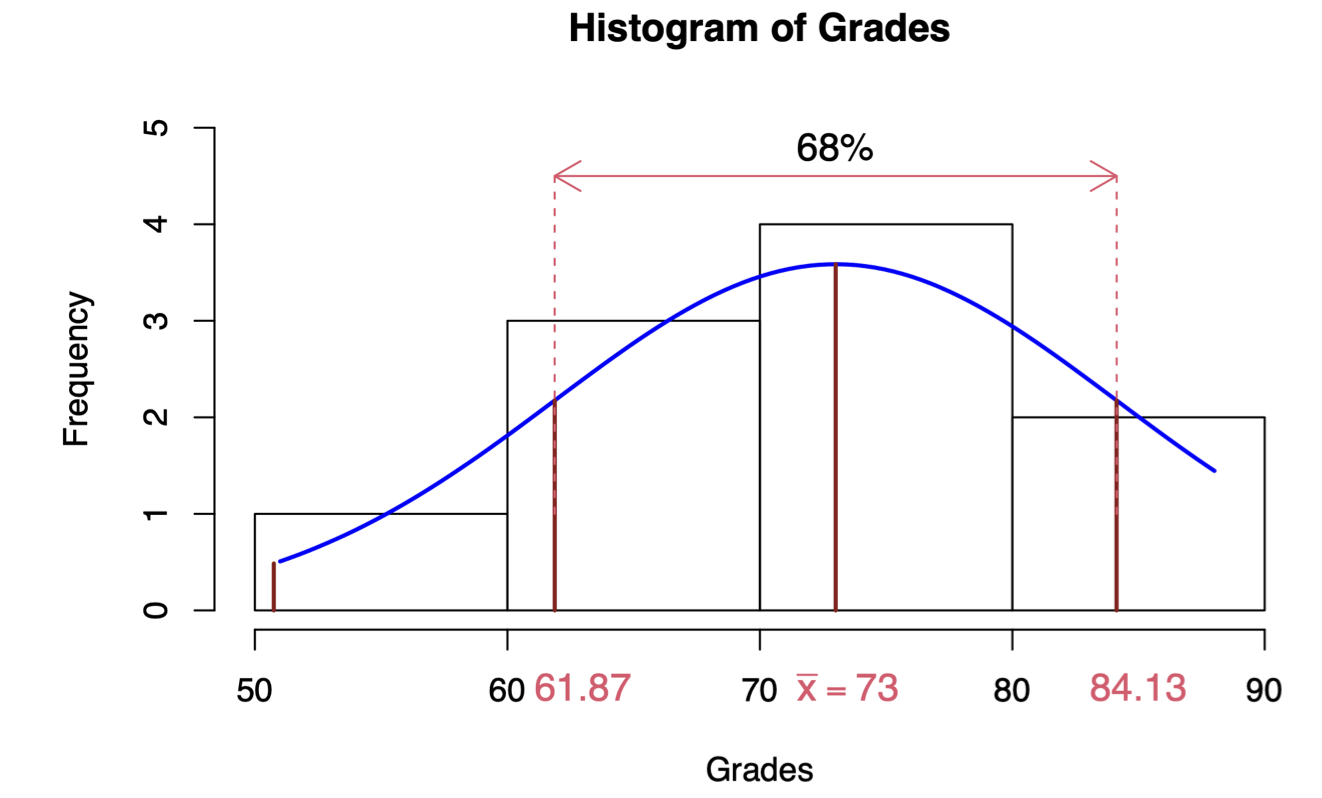
The empirical rule states (for a normally distributed data) that 68% of the data falls within one standard deviation; 95% of the data falls within two standard deviations; 99.7% of the data falls within three standard deviations from the mean.
4.8 Measure of Position: \(z\)-score
The \(z\)-score of an observation tells us the number of standard deviations that the observation is from the mean, that is, how far the observation is from the mean in units of standard deviation.
\[z=\frac{x-\bar{x}}{s}\]
As the \(z\)-score has no unit, it can be used to compare values from different data sets or to compare values within the same data set. The mean of \(z\)-scores is 0 and the standard deviation is 1.
Note that \(s>0\) so if \(z\) is negative, the corresponding \(x\)-value is below the mean. If \(z\) is positive, the corresponding \(x\)-value is above the mean. And if \(z=0\), the corresponding \(x\)-value is equal to the mean.
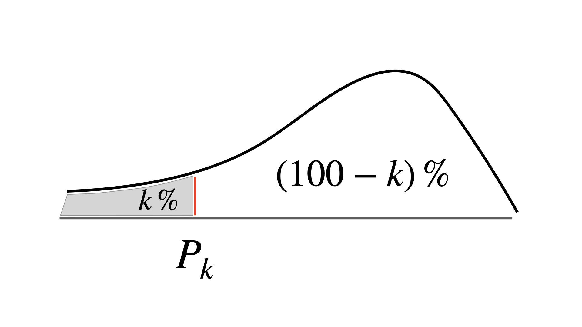
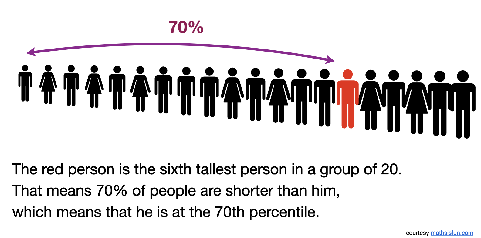
4.9 Percentiles and Quartiles
- Given a set of observations, the \(k\)th percentile, \(P_k\) , is the value of \(X\) such that \(k\)% or less of the observations are less than \(P_k\) and \((100-k)\)% or less of the observations are greater than \(P_k\)
The 25th percentile, \(Q_1\), is often referred to as the first quartile.
The 50th percentile (the median), \(Q_2\), is referred to as the second or middle quartile.
The 75th percentile, \(Q_3\), is referred to as the third quartile
4.9.1 A toy example
4.9.2 The quartiles divide a data set into quarters (four equal parts).
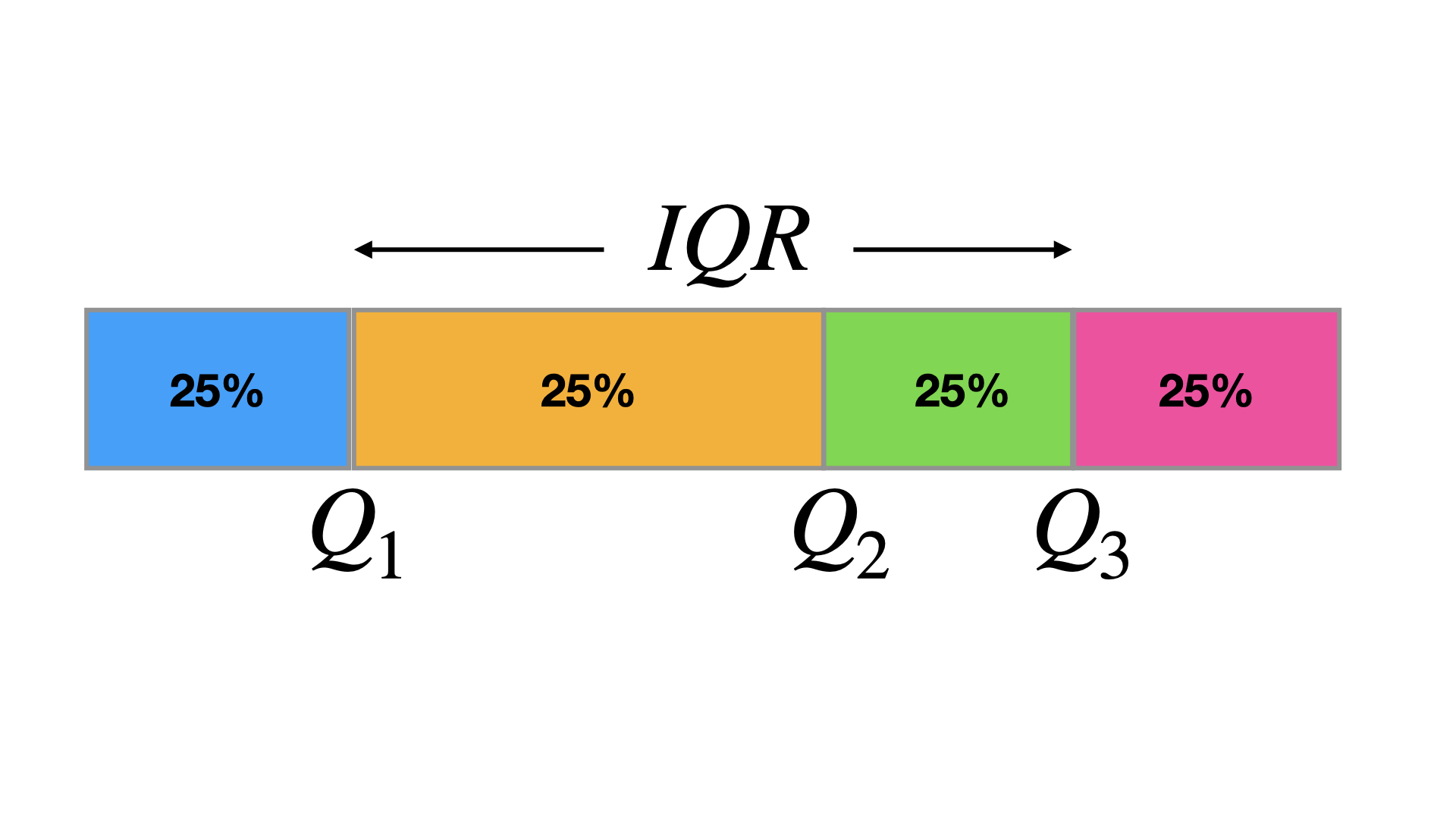
The interquartile range (\(IQR\)) of a data set is the difference between the first and third quartiles (\(IQR = Q_3 - Q_1\))
The IQR is a measure of variation that gives you an idea of how much the middle 50% of the data varies.
4.10 Five-number summary & Boxplots
To graph a boxplot (a box-and-whisker plot), we need the following values (called the five-number summary):
- The minimum entry
- The first quartile \(Q_1\)
- The median (second quartile ) \(Q_2\)
- The maximum entry
- The third quartile \(Q_3\)
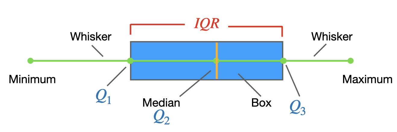 The box represents the interquartile range (\(IQR\)), which contains the middle 50% of values.
4.11 Outliers & Extremes values
Some data sets contain outliers or extremes values, observations that fall well outside the overall pattern of the data. Boxplots can help us to identify such values if some rules-of-thumb are used, e.g.:
Outlier: Cases with values between 1.5 and 3 box lengths (the box length is the interquartile range) from the upper or lower edge of the box.
Extremes: Cases with values more than 3 box lengths from the upper or lower edge of the box.
4.12 Descriptive statistics for qualitative variables
Frequency distributions are tabular or graphical presentations of data that show each category for a variable and the frequency of the category’s occurrence in the data set. Percentages for each category are often reported instead of, or in addition to, the frequencies.
The Mode can be used in this case as a measure of central tendency.
Bar charts and Pie charts are often used to display the results of categorical or qualitative variables. Pie charts are more useful for displaying results of variables that have relatively few categories, in that pie charts become cluttered and difficult to read if variables have many categories.
4.13 Example: Accounting final exam grades
The accounting final exam grades of 10 students are: 88, 51, 63, 85, 79, 65, 79, 70, 73, and 77. Their study programs, respectively, are: MA, MA, MBA, MBA, MBA, MBA, MBA, MSc, MSc, and MSc.
The sample mean grade is \[\bar{x}=\frac{1}{n}\sum_{i=1}^{n}x_i=\frac{1}{10}(88+51+\ldots+77)=73\]
Next we arrange the data from the lowest to the largest grade: 51, 63, 65, 70, 73, 77, 79, 79, 85, 88. The median grade is 75, which located midway between the 5th and 6th ordered data points \((73+77)/2=75\).
The mode is 79 since it appears twice and all other grades appeared only once.
The range is \(88-51=37\).
The variance \[s^2=\frac{1}{n-1}\sum_{i=1}^{n}(x_i-\bar{x})^2=\frac{1}{9}((88-73)^2+\ldots+(77-73)^2)=123.78\]
The standard deviation: \(s=\sqrt{123.78}=11.13\)
The coefficient of variation: \(CV=s/\bar{x}=11.13/73=0.1525\)
Empirical rule: the empirical rule states (for a normally distributed data) that 68% of the data falls within one standard deviation from the mean. In our example, this means that 68% of the grades fall between 61.87 and 84.13 (\(73\pm 11.12555\))
\(~\)
# R codes for "Accounting final exam grades" example
# Data example
grades<-c(88,51,63,85,79,65,79,70,73,77)
program<-factor(c("MA","MA","MBA","MBA","MBA","MBA","MBA","MSc","MSc","MSc"))

# no of observations
length(grades)
## [1] 10# Mean, Median, Variance, standard deviation, range, quantile
mean(grades)## [1] 73median(grades)## [1] 75var(grades)## [1] 123.7778sd(grades)## [1] 11.12555range(grades)## [1] 51 88quantile(grades,probs=c(0,0.25,0.5,0.75,1))## 0% 25% 50% 75% 100%
## 51.00 66.25 75.00 79.00 88.00# Summary
summary(grades)## Min. 1st Qu. Median Mean 3rd Qu. Max.
## 51.00 66.25 75.00 73.00 79.00 88.00# Calculate z-score
(grades-mean(grades))/sd(grades)## [1] 1.3482484 -1.9774310 -0.8988323 1.0785987 0.5392994 -0.7190658
## [7] 0.5392994 -0.2696497 0.0000000 0.3595329scale(grades)## [,1]
## [1,] 1.3482484
## [2,] -1.9774310
## [3,] -0.8988323
## [4,] 1.0785987
## [5,] 0.5392994
## [6,] -0.7190658
## [7,] 0.5392994
## [8,] -0.2696497
## [9,] 0.0000000
## [10,] 0.3595329
## attr(,"scaled:center")
## [1] 73
## attr(,"scaled:scale")
## [1] 11.12555\(~\)
#  Histograms present frequencies for values grouped into interval.
hist(grades,xlab="grades", main="Histogram of grades")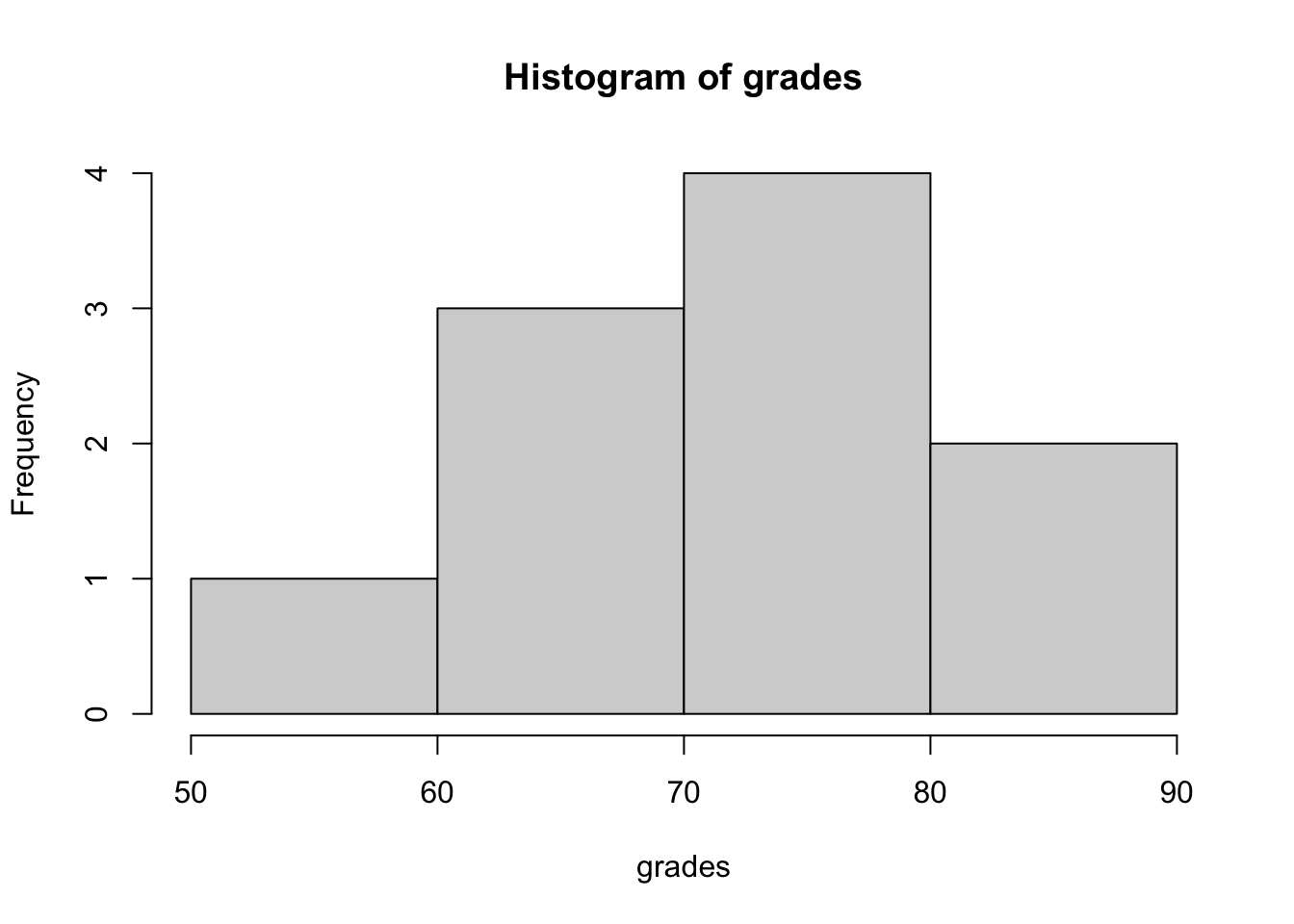
# Boxplot
boxplot(grades,xlab="grades")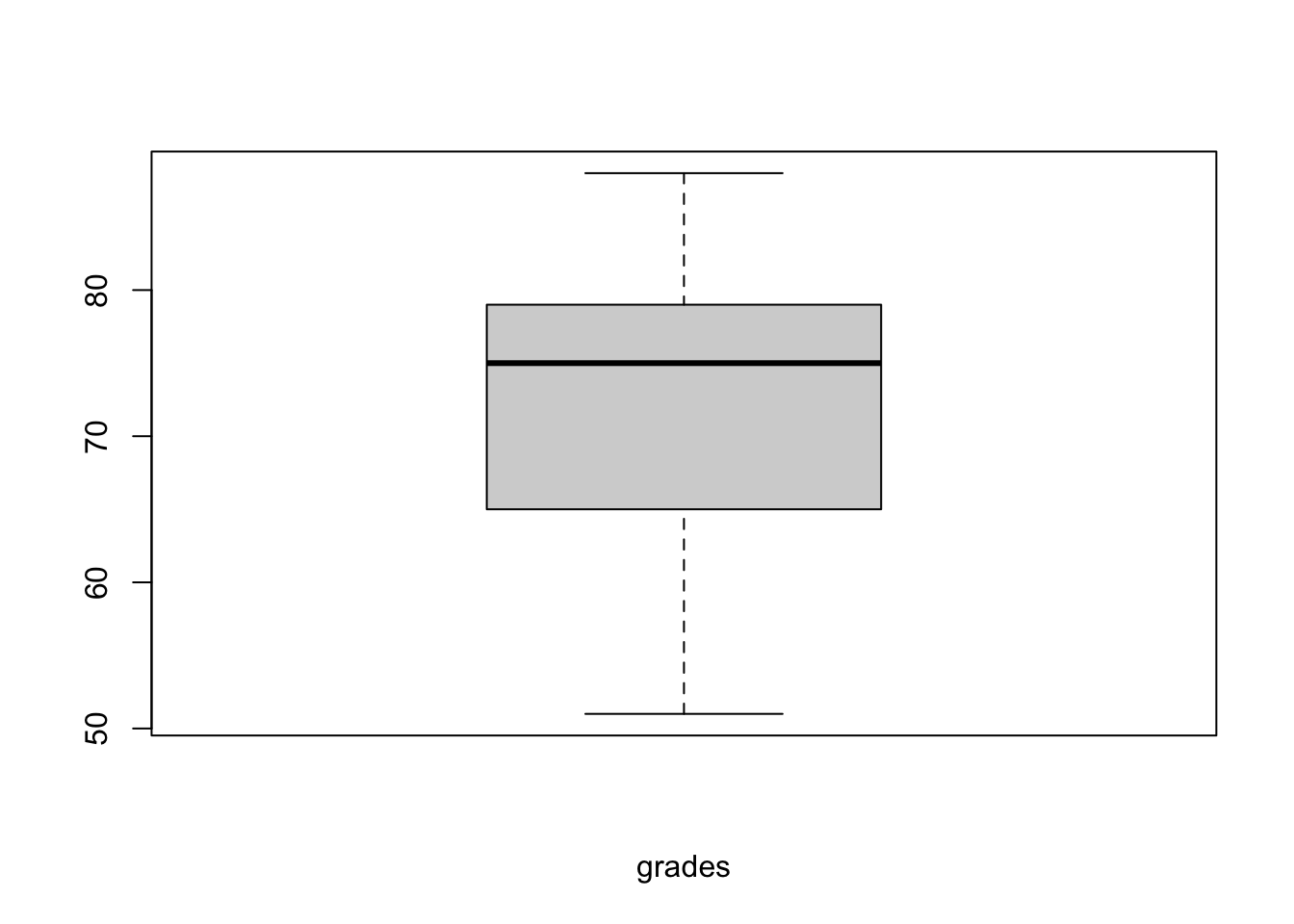
\(~\)
Stem-and-leaf plots: each score on a variable is divided into two parts, the stem gives the leading digits and the leaf shows the trailing digits.
The accounting final exam grades (arranged from the lowest to the largest grade) are: 51, 63, 65, 70, 73, 77, 79, 79, 85, 88.
\(~\)
# Stem-and-leaf plot.
stem(grades)
##
## The decimal point is 1 digit(s) to the right of the |
##
## 5 | 1
## 6 | 35
## 7 | 03799
## 8 | 58Dot plot: is a simple graph to show the relative positions of the data points.
col2<-as.character(factor(program,labels=c("red","blue","orange")))
dotchart(grades, labels=factor(1:10), groups=program, pch=16, col=col2, xlab="Grades",xlim=c(45,100))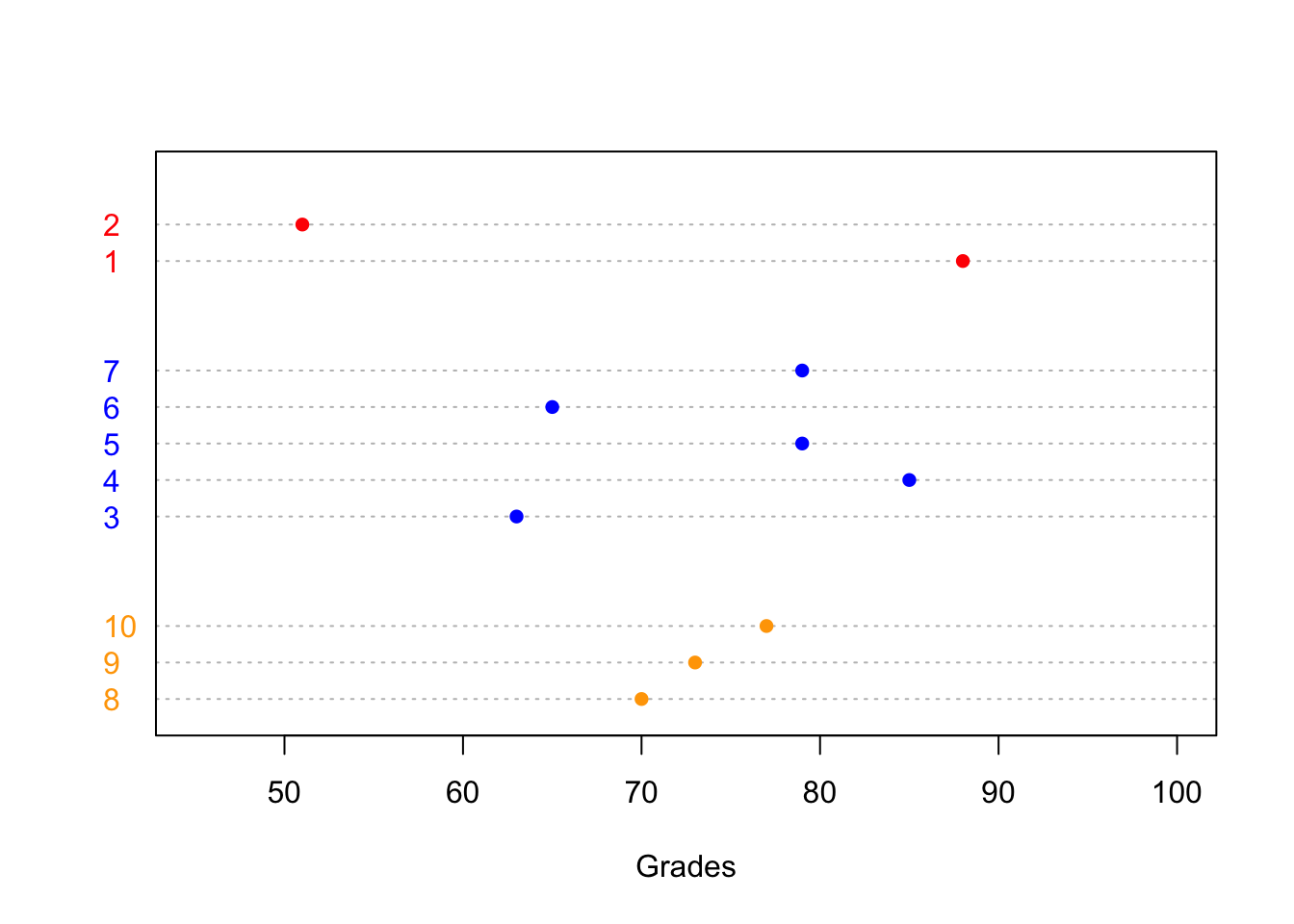
\(~\)
# Frequency table
table(program)
## program
## MA MBA MSc
## 2 5 3# Pie and Bar charts
pie(table(program))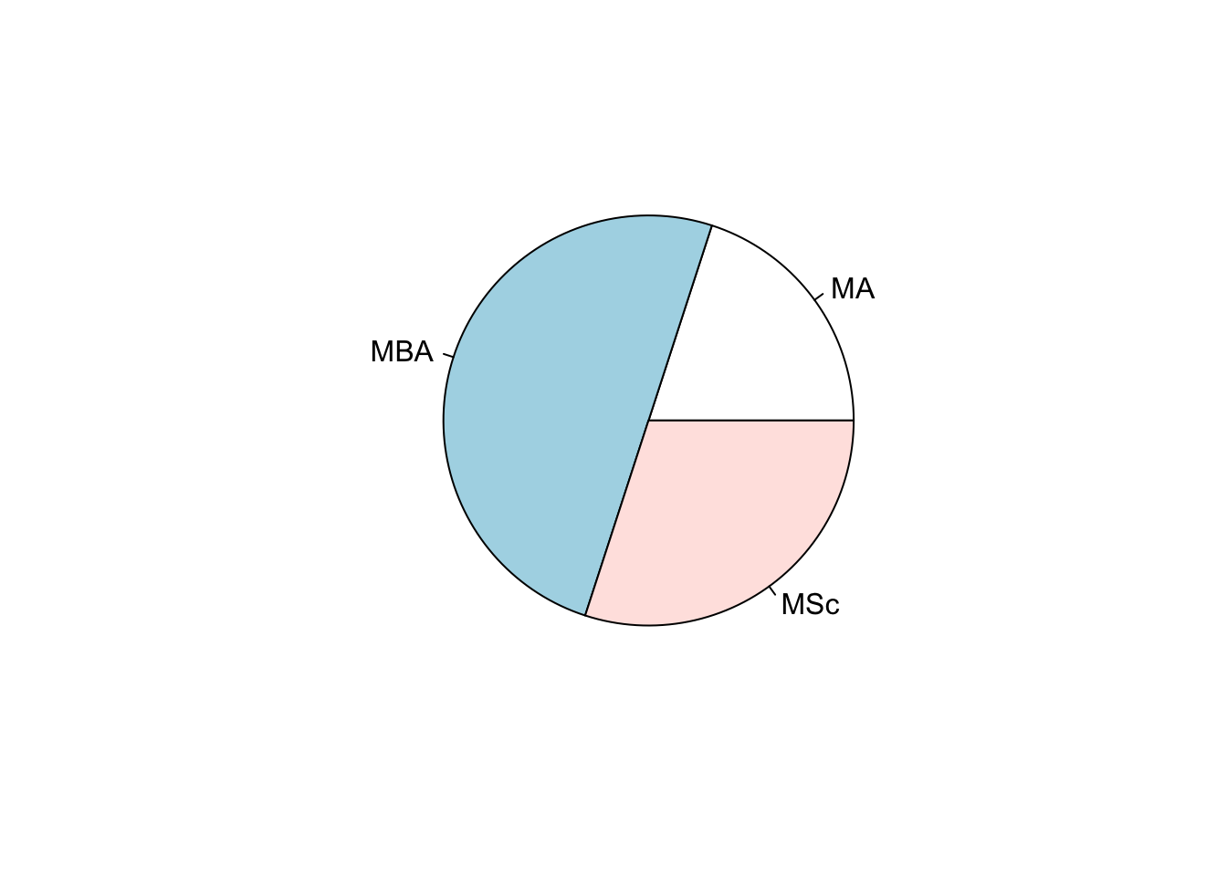
barplot(table(program))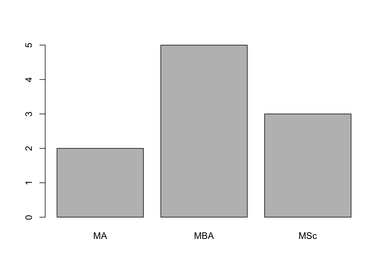
5 Continuous Distributions
5.1 Random Variables
- A random variable is a variable whose possible values are numerical outcomes of a random experiment.
- The term `random’ is used here to imply the uncertainty associated with the occurrence of each outcome.
- Random variables can be either discrete or continuous.
- A realisation of a random variable is the value that is actually observed.
- A random variable is often denoted by a capital letter (say \(X\), \(Y\), \(Z\)) and its realisation by a small letter (say \(x\), \(y\), \(z\)).
5.2 Continuous Random Variables
For a continuous random variable, the role of the probability mass function is taken by a density function, \(f(x)\), which has the properties that \(f(x) \geq 0\) and \[\int_{-\infty}^{\infty} f (x) dx = 1\]
For any \(a < b\), the probability that \(X\) falls in the interval \((a, b)\) is the area under the density function between \(a\) and \(b\): \[P(a < X < b) =\int_{a}^{b} f (x) dx\]
Thus the probability that a continuous random variable \(X\) takes on any particular value is 0: \[P(X = c) =\int_c^c f (x) dx = 0\] %Although this may seem strange initially, it is really quite natural. If the uniform random variable of Example A had a positive probability of being any particular number, it should have the same probability for any number in \([0, 1]\), in which case the sum of the probabilities of any countably infinite subset of \([0, 1]\) (for example, the rational numbers) would be infinite.
If \(X\) is a continuous random variable, then \[P(a < X < b) = P(a \leq X < b) = P(a < X \leq b)\] Note that this is not true for a discrete random variable.
5.3 Cumulative distribution function
The cumulative distribution function (cdf) of a continuous random variable \(X\) is defined as: \[F(x) = P(X \leq x)=\int_{-\infty}^x f (u) du\]
The cdf can be used to evaluate the probability that \(X\) falls in an interval: \[P(a \leq X \leq b) = \int_a^b f (x) dx = F(b) - F(a)\]
5.4 Characteristics of probability distributions
If X is a continuous random variable with density \(f (x)\), then \[\mu= E(X) =\int_{-\infty}^{\infty}x f (x) dx\] or in general, for any function \(g\), \[E(g(X)) =\int_{-\infty}^{\infty}g(x) f (x) dx\]
The variance of \(X\) is \[\sigma^2=Var(X) = E\left\{[X - E(X)]^2\right\}=\int_{-\infty}^{\infty}(x -\mu)^2 f (x) dx\]
The variance of \(X\) is the average value of the squared deviation of \(X\) from its mean.
The variance of \(X\) can also be expressed as \(Var(X)=E(X^2)-[E(X)]^2\) .
5.5 Some useful continuous distributions
5.5.1 Uniform distribution
- A random variable \(X\) with the density function \[f (x) =\frac{1}{b - a},\; a \leq x \leq b\] is called the uniform distribution on the interval \([a,b]\).
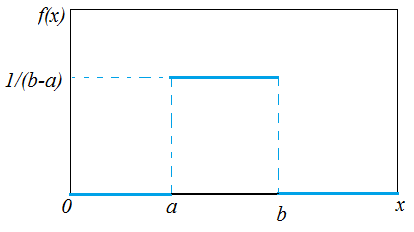
The cumulative distribution function is \[F(x)=\left\{\begin{array}{lll}0& \text{for}& x<a\\ \frac{x-a}{b-a}& \text{for}& a\leq x <b \\ 1&\text{for}& x \geq b\end{array}\right.\]
A special case, \(f (x) = 1\) and \(0 \leq x \leq 1\).
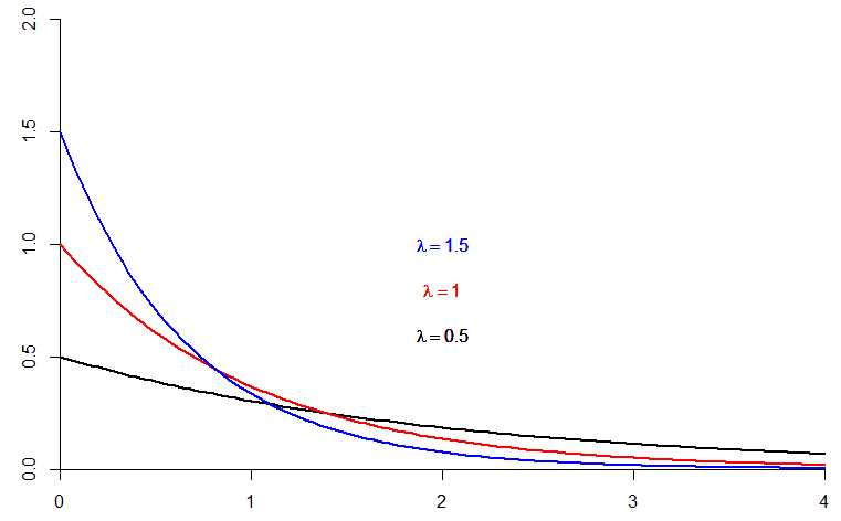
5.5.2 Exponential distribution
- The exponential density function is \[f(x)=\lambda e^{-\lambda x},\; x \geq 0 \;\;\text{and}\;\; \lambda >0\]
- The cumulative distribution function is \[F(x)=\int_{-\infty}^x f(u)du =1-e^{-\lambda x} \]
- The exponential distribution is often used to model lifetimes or waiting times data.
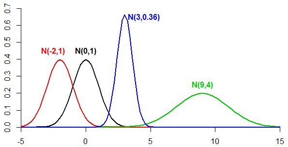
5.5.3 Normal distribution, \(N(\mu,\sigma^2)\)
- The normal (Gaussian) distribution plays a central role in probability and statistics, probably the most widely known and used of all distributions
- The normal distribution fits many natural phenomena, e.g. human’s height, weight, IQ scores. In business, for example, the annual cost of household insurance, among others.
- The density function of the normal distribution depends on two parameters, \(\mu\) and \(\sigma\) (where \(-\infty < \mu < \infty\), \(\sigma > 0\)): \[f (x) = \frac{1}{\sigma \sqrt{2\pi}} e^{-(x-\mu)^2/2\sigma^2}, -\infty<x<\infty\]
- The parameters \(\mu\) and \(\sigma\) are the mean and standard deviation of the normal density.
- We write \(X \sim N(\mu, \sigma^2)\) as short way of saying `\(X\) follows a normal distribution with mean \(\mu\) and variance \(\sigma^2\)’.
5.5.4 Standard normal distribution \(N(\mu=0,\sigma^2=1)\)
- The probability density function of the standardized normal distribution is given by:
\[f (z) = \frac{1}{\sqrt{2\pi}} e^{-z^2/2}, -\infty<z<\infty\]
We write \(Z \sim N(0,1)\) as short way of saying `\(Z\) follows a standard normal distribution with mean 0 and variance 1’.
To standardize any variable \(X\) (into \(Z\)) we calculate \(Z\) as: \[ Z = \frac{X - \mu} { \sigma}\] The \(Z\)-score calculated above indicates how many standard deviations \(X\) is from the mean.

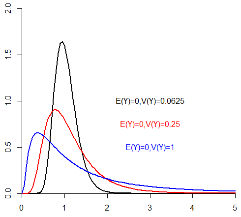
5.5.5 Log-normal distribution and its properties
If \(X\sim N(\mu, \sigma^2)\) then \(Y=e^X\) (\(y \geq 0\)) has a log-normal distribution with mean \(E(Y)=e^{\mu+\sigma^2/2}\) and variance \(V(Y)=(e^{\sigma^2}-1)e^{2\mu+\sigma^2}\).
5.5.6 Distributions derived from the normal distribution
We consider here 3 probability distributions derived from the normal distribution:
- Chi-square distribution
- \(T\) or \(t\) distribution
- \(F\) distribution
These distributions are mainly useful for statistical inference, e.g. hypothesis testing and confidence intervals (to follow).
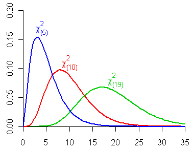
5.5.7 Chi-square distribution, \(\chi^2_{(df)}\)
- If \(Z\) is a standard normal random variable, the distribution of \(U=Z^2\) is called the chi-square distribution with 1 degree of freedom and is denoted by \(\chi^2_1\).
- If \(U_1, U_2,\ldots, U_n\) are independent chi-square random variables with 1 degree of freedom, the distribution of \(V=U_1+ U_2+\ldots+ U_n\) is called the chi-square distribution with \(n\) degrees of freedom and is denoted by \(\chi^2_n\).
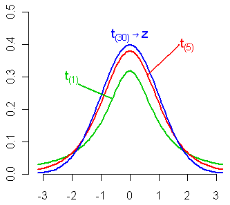
5.5.8 \(T\) distribution, \(t_{(df)}\)
If \(Z \sim N(0,1)\) and \(U \sim \chi^2_n\) and \(Z\) and \(U\) are independent, then the distribution of \(Z/\sqrt{U/n}\) is called the \(t\) distribution with \(n\) degrees of freedom.
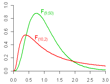
5.5.9 \(F\) distribution, \(F_{(df_1,df_2)}\)
Let \(U\) and \(V\) be independent chi-square random variables with \(m\) and \(n\) degrees of freedom, respectively. The distribution of \[W=\frac{U/m}{V/n}\] is called the \(F\) distribution with \(m\) and \(n\) degrees of freedom and is denoted by \(F_{m,n}\).
5.5.10 Example
- If \(f_X\) is a normal density function with parameters \(\mu\) and \(\sigma\), then
\[f_Y (y) = \frac{1}{a\sigma\sqrt{2\pi }}exp\left[-\frac{1}{2}\left(\frac{y-b-a\mu}{a\sigma}\right)^2\right]\]
Thus, \(Y = aX + b\) follows a normal distribution with parameters \(a \mu + b\) and \(a\sigma\).
If \(X \sim N(\mu, \sigma^2)\) and \(Y = aX + b\), then \(Y \sim N(a \mu + b, a^2\sigma^2)\).
Can you use this to show that \(Z\sim N(0,1)\)?
5.6 Joint distribution
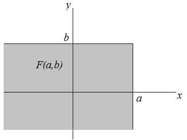
- The joint behaviour of two random variables, \(X\) and \(Y\), is determined by the cumulative distribution function, \[F(x,y)=P(X\leq x, Y \leq y)\] regardless of whether \(X\) and \(Y\) are continuous or discrete. The cdf gives the probability that the point \((X,Y)\) belongs to a semi-infinite rectangle in the plane.
The joint density function \(f(x,y)\) of two continuous random variables \(X\) and \(Y\) is such that \[f(x,y) \geq 0\] \[\int_{-\infty}^{\infty}\int_{-\infty}^{\infty}f(x,y)\;dxdy=1\] \[\int_{c}^{d}\int_{a}^{b}f(x,y)dxdy=P(a \leq X \leq b, c \leq Y \leq d )\] The marginal density function of \(X\) is \[f_X(x)=\int_{-\infty}^{\infty}f(x,y)\;dy\] Similarly, the marginal density function of \(Y\) is \[f_Y(y)=\int_{-\infty}^{\infty}f(x,y)\;dx\]
The cdf of two continuous random variables \(X\) and \(Y\) can be obtained as \[F(x,y)=\int_{-\infty}^{x}\int_{-\infty}^{y}f(u,v)dudv\] and \[f(x,y)=\frac{\partial^2}{\partial x \partial y}F(x,y)\] wherever the derivative is defined.
5.7 Conditional probability (density) function, PDF
- The conditional probability (density) functions may be obtained as follows: \[f_{X|Y}(x|y)=\frac{f(x,y)}{f(y)}\;\;\;\text{conditional PDF of $X$}\] \[f_{Y|X}(y|x)=\frac{f(x,y)}{f(x)}\;\;\;\text{conditional PDF of $Y$}\]
- Two random variables \(X\) and \(Y\) are statistically independent if and only if \[f(x,y)=f(x)f(y)\] That is, if the joint PDF can be expressed as the product of the marginal PDFs. So, \[f_{X|Y}(x|y)=f(x)\;\;\text{and}\;\;f_{Y|X}(y|x)=f(y)\]
5.8 Properties of Expected values and Variance
The expected value of a constant is the constant itself, i.e. if \(c\) is a constant, \(E(c)=c\).
The variance of a constant is zero, i.e. if \(c\) is a constant, \(Var(c)=0\).
If \(a\) and \(b\) are constants, and \(Y = aX + b\), then \(E(Y)=a E(X)+b\) and \(Var(Y) = a^2Var(X)\) (if \(Var(X)\) exists).
If \(X\) and \(Y\) are independent, then \(E(XY) = E(X)E(Y)\) and \[Var(X+ Y)=Var(X) + Var(Y)\] \[Var(X- Y)=Var(X) + Var(Y)\]
If \(X\) and \(Y\) are independent random variables and \(g\) and \(h\) are fixed functions, then \[E[g(X)h(Y )] = E[g(X)]E[h(Y )]\]
5.9 Covariance
- Let \(X\) and \(Y\) be two random variables with means \(\mu_x\) and \(\mu_y\), respectively. Then the covariance between the two variables is defined as \[cov(X,Y)=E\left\{(X-\mu_x)(Y-\mu_y)\right\}=E(XY)-\mu_x\mu_y\]
- If \(X\) and \(Y\) are independent, then \(cov(X,Y)=0\).
- If two variables are uncorrelated, that does not in general imply that they are independent.
- \(Var(X)=cov(X,X)\)
- \(cov(bX+a, dY+c)=bd\; cov(X,Y)\), where \(a,b,c\), and \(d\) are constants.
5.10 Correlation Coefficient
- The (population) correlation coefficient \(\rho\) is defined as \[\rho=\frac{cov(X,Y)}{\sqrt{Var(X)Var(Y)}}=\frac{cov(X,Y)}{\sigma_x \sigma_y}\]
- Thus, \(\rho\) is a measure of linear association between two variables and lies between \(-1\) (indicating perfect negative association) and \(+1\) (indicating perfect positive association).
- \(cov(X,Y)=\rho \;\sigma_x \sigma_y\)
- Variances of correlated variables, \[Var(X\pm Y)=Var(X)+Var(Y) \pm 2 cov(X,Y)\] \[Var(X\pm Y)=Var(X)+Var(Y) \pm 2 \rho\; \sigma_x \sigma_y\]
5.11 Conditional expectation and conditional variance
Let \(f(x,y)\) be the joint PDF of random variables \(X\) and \(Y\). The conditional expectation of \(X\), given \(Y=y\), is defined as \[E(X|Y=y)=\sum_x x f_{X|Y}(x|Y=y)\;\;\; \text{if $X$ is discrete}\] \[E(X|Y=y)=\int_{-\infty}^{\infty} x f_{X|Y}(x|Y=y)dx\;\;\; \text{if $X$ is continuous}\] The conditional variance of \(X\) given \(Y=y\) is defined as, if \(X\) is discrete, \[Var(X|Y=y)=\sum_x [X-E(X|Y=y)]^2 f_{X|Y}(x|Y=y)\] and if \(X\) is continuous, \[Var(X|Y=y)=\int_{-\infty}^{\infty} [X-E(X|Y=y)]^2 f_{X|Y}(x|Y=y)dx\]